Series Review
One of the early stages of creating any Power BI report is the development of the data model. The data model will consist of data tables, relationships, and calculations. There are two types of calculations: calculated columns, and measures.
Check out Power BI Row Context: Understanding the Power of Context in Calculations for key differences between calculated columns and measures.

Power BI Row Context: Understanding the Power of Context in Calculations
Row Context — What it is, When is it available, and its Implications
All expressions, either from a calculated column or a measure, get evaluated within the evaluation context. The evaluation context limits the values in the current scope when evaluating an expression. The filter context and/or the row context make up the evaluation context.
Power BI Row Context: Understanding the Power of Context in Calculations explores the row context in depth. While Power BI Iterators: Unleashing the Power of Iteration in Power BI Calculations explores iterator functions, which are functions that create row context.

Power BI Iterators: Unleashing the Power of Iteration in Power BI Calculations
Iterator Functions — What they are and What they do
This article is the third of a Power BI Fundamental series with a focus on the filter context. The example file used in this post is located here – GitHub.
Introduction to Filter Context
Filter context refers to the filters applied before evaluating an expression. This filter context limits the set of rows of a table available to the calculation. There are two types of filters to consider, the first is implicit filters or filters applied by the user via the report canvas. The second type is explicit filters which use functions such as CALCULATE() or CALCULATETABLE().
The applied filter context can contain one or many filters. When there are many filters the filter context will be the intersection of all the filters. When the filter context is empty all the data is used during the evaluation.
The filter context does not iterate — this is a key difference between the filter context and the row context
Filter context propagates through the data model relationships. When defining each model relationship the cross-filter direction is set. This setting determines the direction(s) the filters will propagate. The available cross-filter options depend on the cardinality type of the relationship. See available documentation for more information on Cross-filter Direction and Enabling Bidirectional Cross-filtering.
It is important to be familiar with certain DAX functions which can modify the filter context. Some examples used in the post include CALCULATE(), ALL(), and FILTER().
The CALCULATE Function
The CALCULATE() function can add filters to a measure expression, ignore filters applied to a table, or overwrite filters applied from within the report visuals. The CALCULATE() function is a powerful and important tool when updating or modifying the filter context.
The syntax of CALCULATE() is:
CALCULATE(<expression>, <filter1>, <filter2>, ...)
Use the CALCULATE() function when modifying the filter context of an expression that returns a scalar value. Use CALCULATETABLE() when modifying the filter context of an expression that returns a table.
Exploring Filter Context
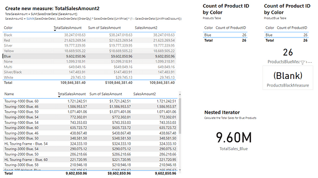
The table below is a visualization of the total sales amount for each product color.
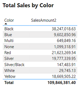
The table visual creates filter context, as seen by the total sales amount for each color or row. Evaluating SalesAmount2 occurs by first filtering the SalesOrderDetail table by the color, and then evaluating the measure with the filtered table. This is then repeated for each product color in the SalesOrderDetail table.
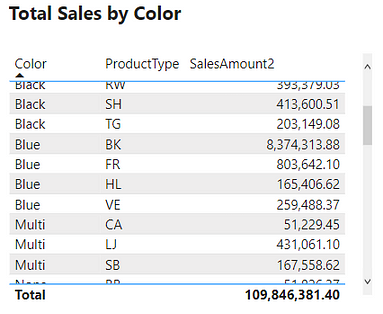
The above example only contained the single product color filter. However, as mentioned previously, the filter context can contain multiple filters. The example table below adds the ProductType to the table. The addition of this field breaks down the total sales first by color and then by product type. For each row, the underlying SalesOrderDetail table is first filtered by color and product type before evaluating the SalesAmount2 measure. In these examples, it is the table visual that is creating the filter context.
Create Filter Context with Slicers
Another way to create filter context is through the use of slicer visuals. For this example, a slicer of the ProductType is created.
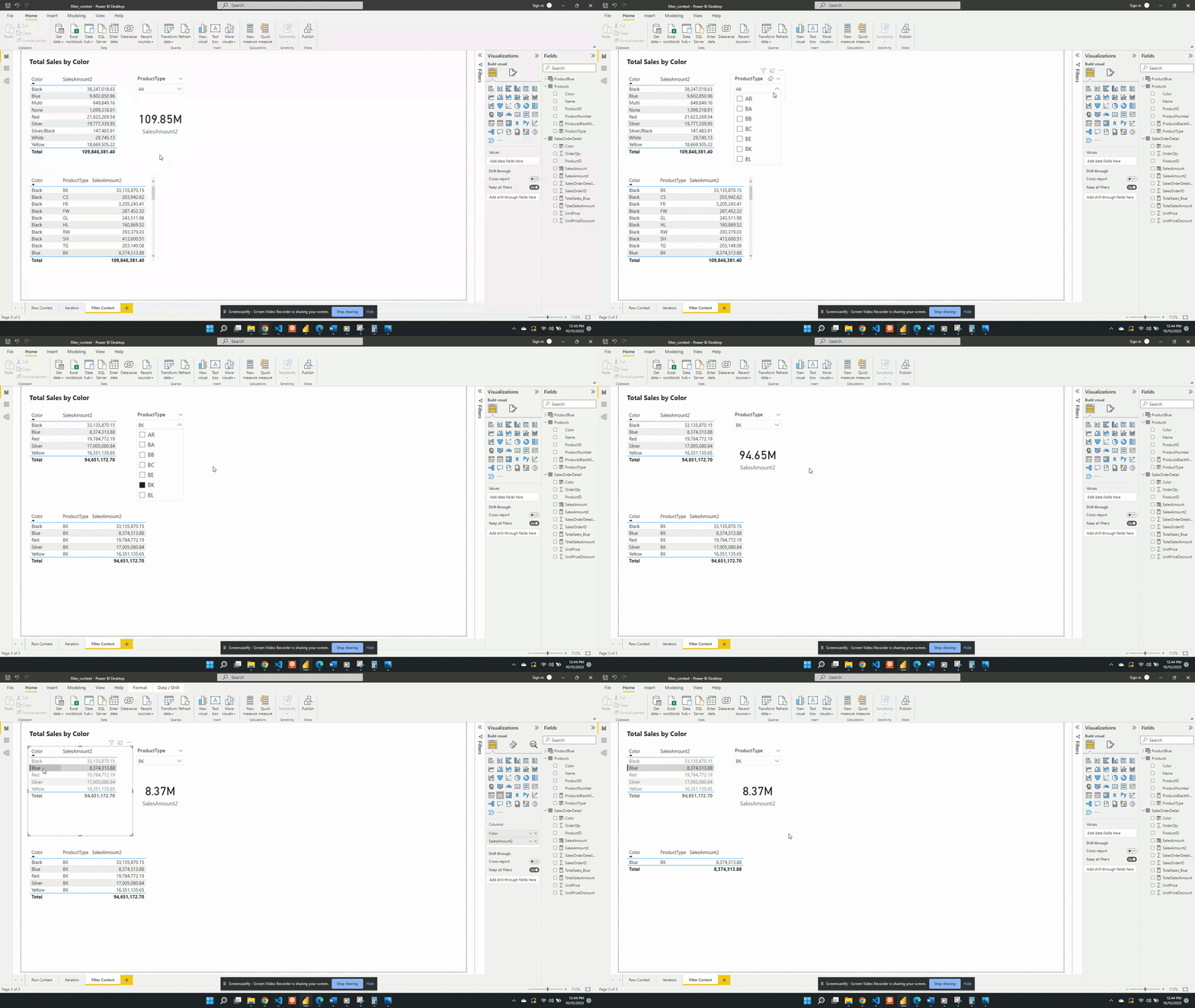
When no value is selected in the slicer the filter context from the slicer visual is null. Meaning at first the card visual shows the SalesAmount2 value evaluated for all data. Additionally, when no value is selected in the slicer the only filter context is ProductColor from the table visual.
Following the selection of BK in the product type slicer, the values in both the table and the card visual are updated. The card visual now has one filter context which is the product type BK. This is evaluated by creating a filtered table and SalesAmount2 is evaluated for this filtered table.
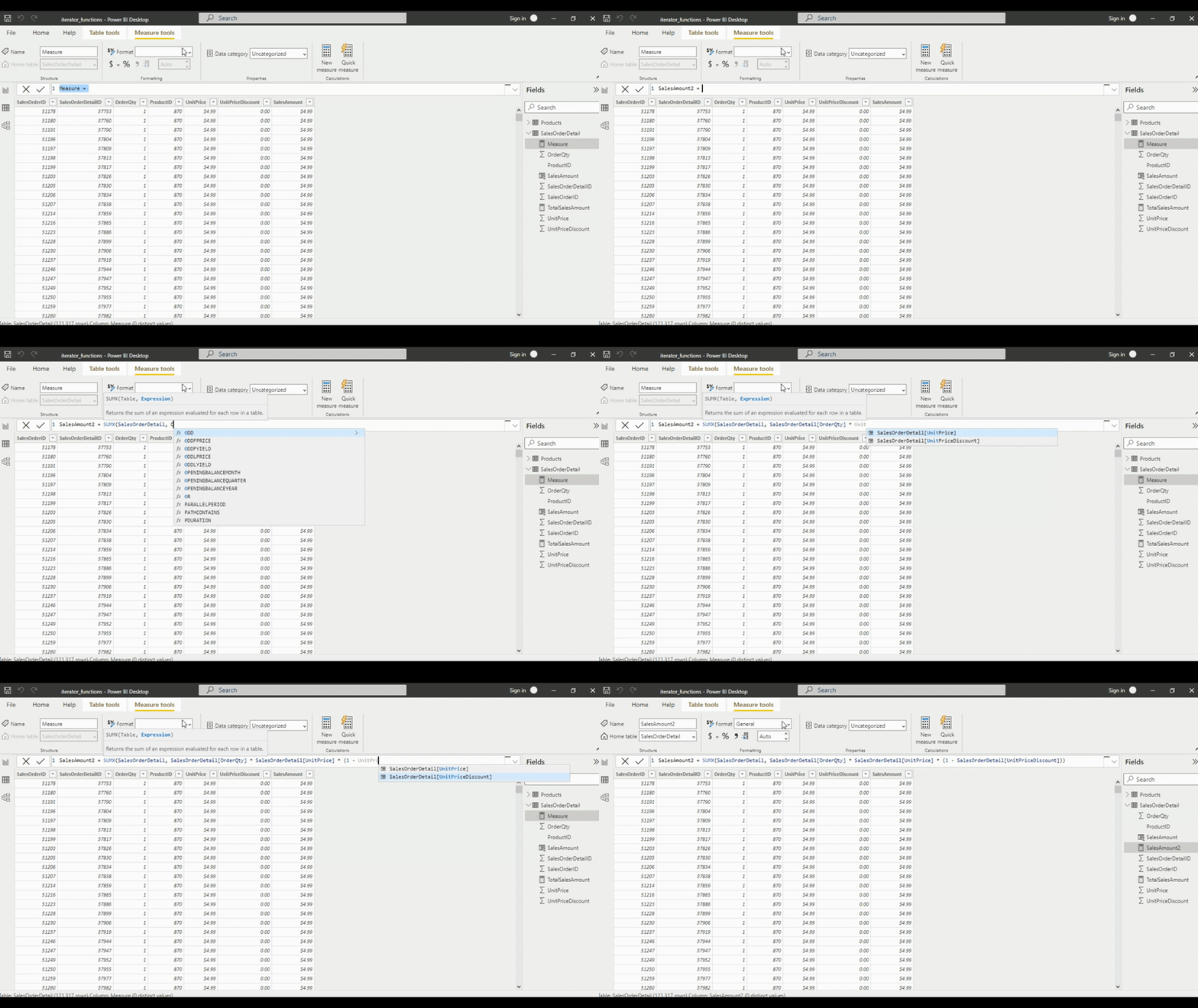
The SalesAmount2 measure is defined by:
SalesAmount2 =
SUMX (
    SalesOrderDetail,
    SalesOrderDetail[OrderQty] * SalesOrderDetail[UnitPrice] *
    ( 1 - SalesOrderDetail[UnitPriceDiscount] )
)
After selecting an option from the slicer the measure is re-evaluated. The re-evaluation occurs to account for the newly created filter context. The filter context creates a subset of the SalesOrderDetail table that matches the slicer selection. Then the row context evaluates the expression row-by-row for the filtered table and is summed. SUMX() is an example of an iterator function, see Power BI Iterators: Unleashing the Power of Iteration in Power BI Calculations for more details. The updated value is then displayed on the card visual.

Power BI Iterators: Unleashing the Power of Iteration in Power BI Calculations
Iterator Functions — What they are and What they do
The table visual works in a similar fashion but, there are two filters applied. The table visual has an initial filter context of the product color. After the selection of BK, the table gets updated to visualize the intersection of the product color filter and the product type filter.
Following a selection in the slicer visual, if a row in the table visual is selected this will also apply a filter. The filter context is the intersection of the table selection filters and the slicer. The updated filter context gets applied to all other visuals (e.g. the card visual).
The filter context can contain one or many filters. The filter can come from one or many visuals and gets applied before evaluating the expression. Meaning the filter context gets applied before using the row context to evaluate an expression row-by-row
Create Filter Context with CALCULATE
Previous examples created the filter context using implicit filters. Generally, the user creates this type of filter through the user interface. Another way to create filter context is by using explicit filters. Explicit filters get created through the use of functions such as CALCULATE(). For this example, rather than having to select BK in the slicer to view total bike sales, we will use CALCULATE(). We will create a new measure that will force the filter context. We can do this because CALCULATE() allows us to set the filter context for an expression.
We define the BikeSales measure as:
BikeSales =
CALCULATE (
   SalesOrderDetail[SalesAmount2],
   Products[ProductType] = "BK"
)
- Expression:
SalesOrderDetails[SalesAmount2] - Filter:
Products[ProductType]="BK"
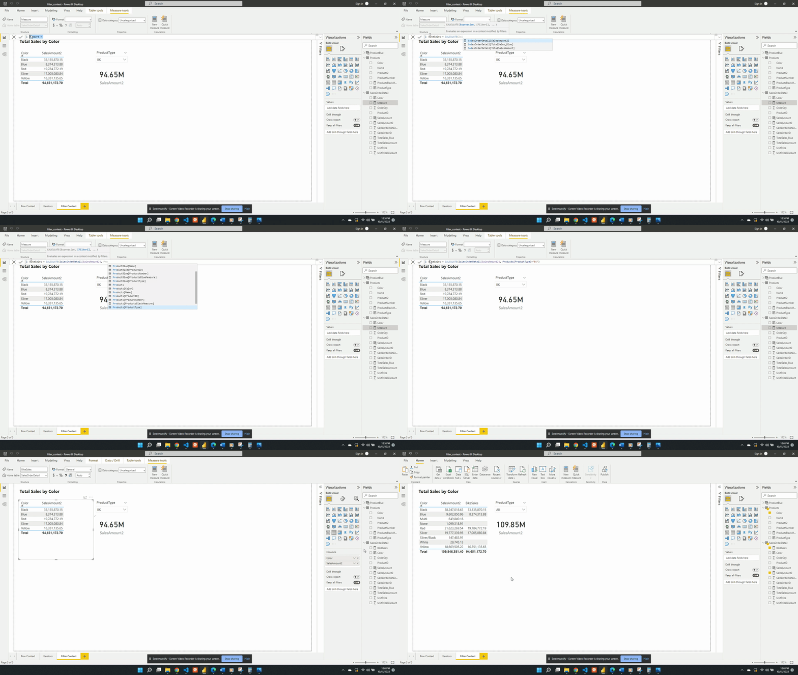
BikeSales is then added to the table visual alongside SalesAmount2. When the BK product type is the slicer selection the two table columns are equal. Both measures have the same filter context created by product color and product type. Removing the implicit product type filter by unselecting a product type updates the filter context. The SalesAmount2 expression is re-evaluated with the updated filter context. Since the filter context created by the slicer is now null the SalesAmount2 value calculates using all the data. The BikeSales values do not change. This is because of the explicit filter used by the CALCULATE() function when we defined the measure. The BikeSales measure still has the filter Products[ProductType]="BK" applied regardless of the product type slicer.
The CALCULATE() function only creates filter context and does not create row context. So an important question to ask is why or how the BikeSales measure works. The CALCULATE() function references a specific column value, Products[ProductType]="BK". Yet, the CALCULATE() function does not have row context. So how does Power BI know which row it is working with? The answer is that the CALCULATE() function applies the FILTER() function. And the FILTER function creates the row context required to evaluate the measure.
Within the CALCULATE() function the Products[ProductType]="BK filter is shorten syntax. The filter argument passed to CALCULATE() is equivalent to FILTER(ALL(Products[ProductType]), Products[ProductType]="BK")). The ALL() function removes any external filters on the ProductType column and is another example of a function that can modify the filter context.
Keep External filters with CALCULATE
The CALCULATE() function evaluates the filter context both outside of and within the function. The filter context outside of the function can come from user interaction with visuals. The filter context within the function is the filter expression(s).
CALCULATE() overwrites external filters or filters that are outside of the function
To explore this we create a table with the Product Type, SalesAmount2, and SalesBike.
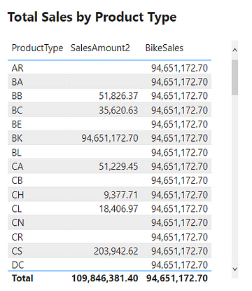
The SalesAmount2 column shows the total sales amount, if any, as expected. While the BikeSales column shows the same repeated value for all rows and is incorrect. Looking at the Product Type BK row we can see this row is correct. This table demonstrates that CALCULATE()overwrites external filters.
For example, the BB product type row filters SalesOrderDetail before evaluating SalesAmount2. This returns the correct total sales for the BB product type. When evaluating BikeSales this external product type filter gets overwritten. The measure calculates the sales amount value for the BK product type due to the explicit filter and returns this value for all rows.
CALCULATE() can be modified to keep both external and internal filters
Using the KEEPFILTERS() function within CALCULATE() will force CALCULATE() to keep both external and internal filters.
To do this we update BikeSales to:
BikeSales =
CALCULATE(
   SalesOrderDetail[SalesAmount2],
   KEEPFILTERS(Products[ProductType]="BK")
)
After updating the measure definition the resulting table is shown below.
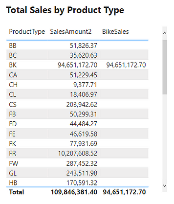
Keeping the external filters is shown by the empty values for all rows except BK. For example, we look again at the BB product type row. When evaluating BikeSales Power BI keeps the external filter Products[ProductType]="BB" and the internal filter Products[ProductType]="BK". When applying more than one filter the filter context is the intersection of the two. The intersection of the two applied filters for the BB row is empty. A product cannot be both of type BB and BK.
More CALCULATE Examples
The CALCULATE() function plays an integral part in the filter context. Below are more examples to show key concepts and show that CALCULATE() is an important part of the filter context.
Creating a measure of High Quantity Sales
For the first example, we will be creating a sales measure showing the total sales amount for high-quantity orders. Creating this measure requires first filtering the SalesOrderDetail table based on the OrderQty. Then evaluating the SalesAmount2 measure with this filtered table.
We define HighQtySales as:
HighQtySales =
CALCULATE(
   [SalesAmount2],
   SalesOrderDetail[OrderQty]>25
)
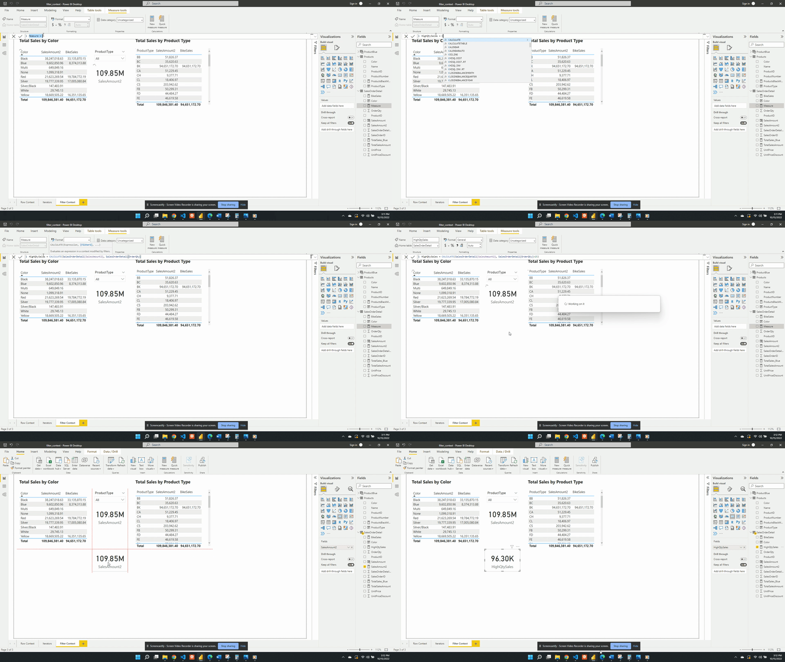
We then visualize this measure on a card visual and see that 96.30K of our total 109.85M sales come from a high-quantity order. This again demonstrates the filter arguments passed to CALCULATE() are shorthand syntax. The filter arguments within CALCULATE() use the FILTER() function to create the row context required. In this example SalesOrderDetail[OrderQty]>25 is equivalent to FILTER(ALL(SalesOrderDetail),SalesOrderDetail[OrderQty] > 25).
The FILTER() function is an example of an iterator function and creates the row context. The row context allows for row-by-row evaluation of the OrderQty. Meaning it evaluates SalesOrderDetail[OrderQty] > 25 for each row of the SalesOrderDetail table. FILTER() then returns a virtual tale that is a subset of the original and contains only orders with a quantity greater than 25.
The CALCULATE() function creates filter context because the filter arguments provide a table. This table is the intersection of all the filter expressions passed to CALCULATE().
Percentage of Sales by Product Color
For the second example, we will create a measure to show the percentage of total sales for each product color. To create this we will start with a new AllSales measure. AllSales uses the CALCULATE() function to remove any filters and evaluates SalesAmount2.
We define AllSales as:
AllSales =
CALCULATE(
   [SalesAmount2],
   ALL(Products[Color])
)
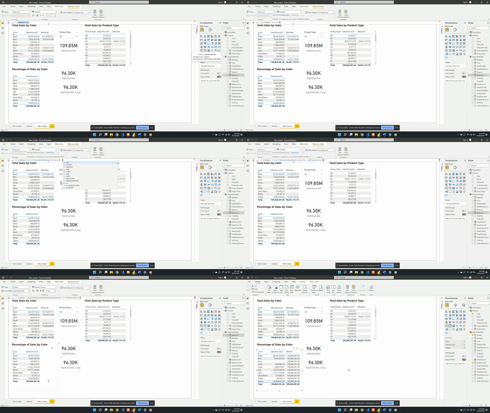
AllSales is then added to the table visual Percentage of Sales by Color. Once added the AllSales column shows 190.85M total sales value for each color. This is consistent with the SalesAmount2 card visual. Repeating this value for each color is also expected because of the filter expression ALL(Products[Color]).
ALL(Products[Color]) creates a new filter context and gets evaluated with any other filters from the visuals. In this example, CALCULATE() overwrites any external filters on Products[Color]. This is why once added to the table visual AllSales displays the total sales value repeated for each row.
The ALL() function removes any filter limiting the color column that may exist while evaluating AllSales. It is best practice to define a measure as specific as possible. Notice, in this example ALL() applies to Product[Color], rather than the entire Product table. If other filters exist on other columns from the visuals these filters will still impact the evaluation. For example, selecting a product type from the slicer will adjust all values.
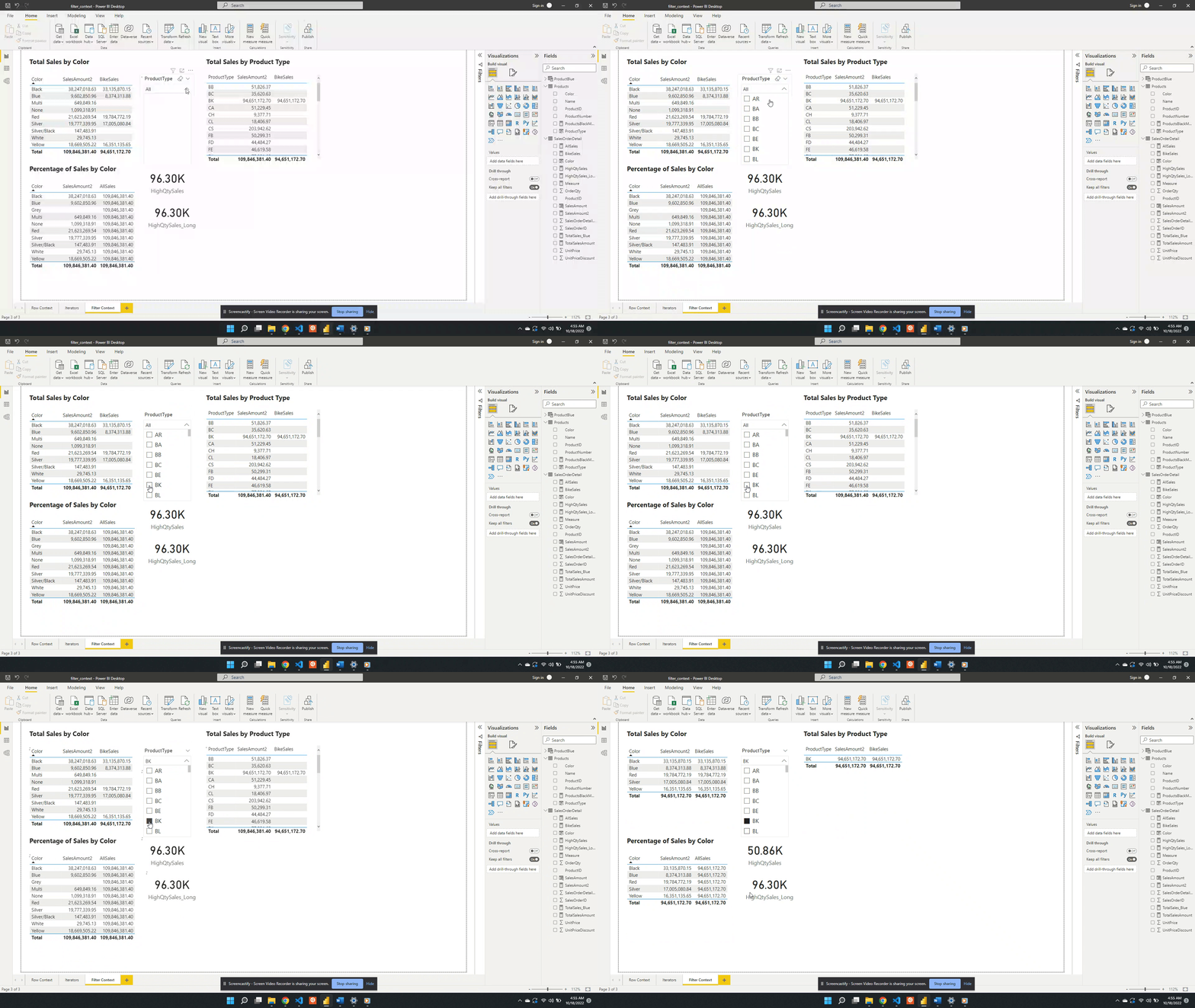
Following the selection, SalesAmount2 represents the total BK sales for each color. While the AllSales measure now represents the total sales for all BK product types. This occurs because when there are multiple filters the result is the intersection of all the filters.
In this case, All(Product[Color]) removes the filter on the color column. The slicer visual creates an external filter context of only BK product types. During the evaluation, the intersection of these two creates the evaluation context.
We can also remove the external filter context created by the product type slicer. To do this, we update the AllSales measure to include Products[ProductType] as an additional filter argument.
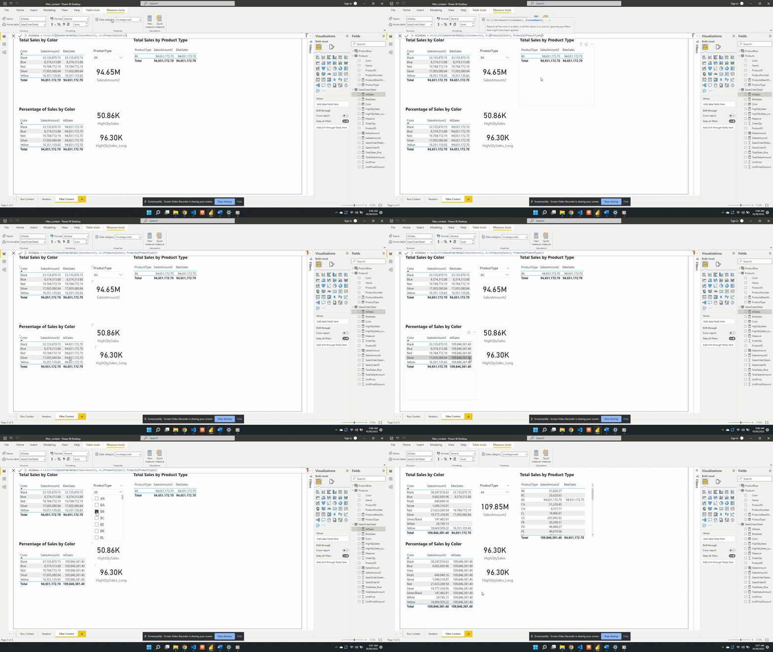
We update the filter expression of the CALCULATE() function to:
AllSales =
CALCULATE(
   [SalesAmount2],
   ALL(Products[Color],
   Products[ProductType]
)
After updating the measure the AllSales column of the table visual updates to the total sales value. The column now displays the expected 109.85M value and is no longer impacted by the filter context created by the slicer visual.
Another option to remove the filter context within CALCULATE() is to use the REMOVEFILTER() function.
AllSales =
CALCULATE(
   SalesOrderDetail[SalesAmount2],
   REMOVEFILTERS(
      Products[Color],
      Products[ProductType]
   )
)
We created AllSales as an initial step of the broader goal to calculate the percentage of total sales. To calculate the percentage we will update the AllSales expression. We can do this by saving the AllSales expression as a variable within the measure. We will also create another variable to store the SalesAmount2 value, which will be the total sales for each product color. Lastly, we will update the measure name to PercentageSales which will RETURN the division of the two sales variables.
PercentageSales =
VAR Sales = SalesOrderDetail[SalesAmount2]
VAR AllSales =
CALCULATE(
   SalesOrderDetail[SalesAmount2],
   REMOVEFILTERS(
      Products[Color],
      Products[ProductType]
   )
)

RETURN
DIVIDE(Sales, AllSales)
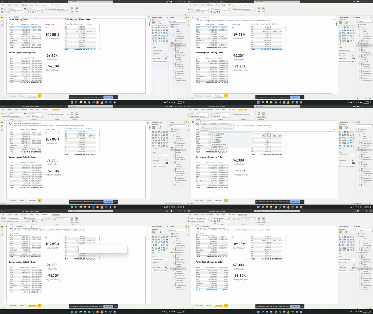
It is best practice to use the DIVIDE function because it provides handling of divide by zero errors and will return a blank or a specified value.
Thank you for reading! Stay curious, and until next time, happy learning.
And, remember, as Albert Einstein once said, “Anyone who has never made a mistake has never tried anything new.” So, don’t be afraid of making mistakes, practice makes perfect. Continuously experiment and explore new DAX functions, and challenge yourself with real-world data scenarios.
If this sparked your curiosity, keep that spark alive and check back frequently. Better yet, be sure not to miss a post by subscribing! With each new post comes an opportunity to learn something new.


