Time Travel in Power BI: Mastering Time Intelligence Functions


The Tools to Time Travel: An Introduction

In Power BI, time intelligence functions are your handy time machines. They enable you to extract useful insights from your data by manipulating time periods. These functions range from calculating sales year-to-date (YTD) to comparing data from previous years. If you want to unlock the true potential of your Power BI reports, you need to harness the might of Time Intelligence functions. In this post, we will unpack six time intelligence functions: DATESYTD, TOTALYTD, SAMEPERIODLASTYEAR, DATEADD, DATESINPERIOD, and DATESBETWEEN.

For those of you eager to start experimenting and diving deeper there is a Power BI report loaded with the sample data used in this post ready for you. So don’t just read, dive in and get hands-on with DAX Functions in Power BI. Check out it here:


The Twin Siblings: DATESYTD and TOTALYTD

First stop on our journey, the twin siblings, DATESYTD and TOTALYTD.

DATESYTD is the Einstein of the Power BI world, it uses the concept of relative time to help us compute values from the start of the year to the last date in the data. The syntax is as simple as the concept:

DATESYTD(dates[, year_end_dates])

Here, dates is a column containing dates, and year_end_date is an optional parameter to specify the year-end date, with a default value of December 31st.

On the other hand, TOTALYTD takes it up a notch. It summarizes data for the same period in a given year. The syntax of this function is:

TOTALYTD(expression, dates[, filter])

In this syntax, expression is what you want to calculate, dates is a column containing dates, and filter is a filter to restrict the calculation over time. TOTALYTD is DATESYTD, but with additional calculation power.

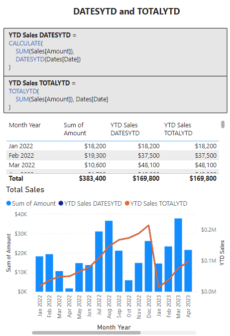
Here are example DAX formulas to calculate the total sales amount from the start of the year till the current date.

YTD Sales DATESYTD =
CALCULATE(
    SUM(Sales[Amount]),
    DATESYTD(Dates[Date])
)

And here is how you can calculate the same using TOTALYTD

YTD Sales TOTALYTD =
TOTALYTD(
  SUM(Sales[Amount]), 
  Dates[Date]
)

While both functions return the same result in this case, the key difference lies in their flexibility. DATESYTD just provides a set of dates, but TOTALYTD goes a step further to calculate an expression over those dates. Notice YTD Sales DATESYTD uses DATESYTD in combination with CALCULATE in order to achieve the same outcome as YTD Sales TOTALYTD.

For more information on these two head over to the Microsoft documentation for DATESYTD and TOTALYTD.

Learn more about: DATESYTD

Learn more about: TOTALYTD


The Cousins: SAMEPERIODLASTYEAR and DATEADD

Next up the cousins, SAMEPERIODLASTYEAR and DATEADD. SAMEPERIODLASTYEAR is the function that does exactly as the name suggests and always knows what happened “this time last year”. This is perfect for spotting trends, analyzing seasonality, or measuring growth. The syntax couldn’t be more straightforward:

SAMEPERIODLASTYEAR(dates)

Here, dates is a column that contains dates. Think of this function as equivalent to you Facebook memories, reminding you of what happened exactly one year ago.

DATEADD is the flexible function that allows you to go back (or forward) any number of intervals you choose. This handy function’s syntax is:

DATEADD(dates, number_of_intervals, interval)

Here, dates is your date column, number_of_intervals is the number of intervals to move (can be negative for moving backwards), interval and is the interval to use (DAY, MONTH, QUARTER, or YEAR). This function lets you journey backward or forward in time with ease!

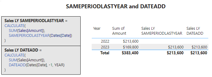
The example for this duo calculates the total sales for the same period in the previous year. The DAX formula for this example is:

Sales LY SAMEPERIODLASTYEAR =
CALCULATE(
    SUM(Sales[Amount]),
    SAMEPERIODLASTYEAR(Dates[Date])
)

Similarly, using DATEADD, you can achieve the same result by subtracting one year from the current date:

Sales LY DATEADD =
CALCULATE(
    SUM(Sales[Amount]),
    DATEADD(Dates[Date], -1, YEAR)
)

While both of these functions seem to do the same job, the difference again lies in their flexibility. SAMEPERIODLASTYEAR only takes you back one year, while DATEADD give you the liberty to move as far back or forward as you want, making it a more flexible option overall.

Visit the Microsoft documentation for SAMEPERIODLASTYEAR and DATEADD for a deeper dive.

Learn more about: SAMEPERIODLASTYEAR

Learn more about: DATEADD


The Mysterious Pair: DATESINPERIOD and DATESBETWEEN

Last but not least, let’s explore the mysterious pair DATESINPERIOD and DATESBETWEEN. DATESINPERIOD has your back if you need to calculate data for a specific period. It returns a table that contains a column of dates that starts from a specific date, extends by a specified interval, and stops at the end of the last interval.

Its syntax is:

DATESINPERIOD(dates, start_date, number_of_intervals, interval)

Here, dates is a column containing dates, start_date is the start date for the calculation, number_of_intervals is the number of intervals to include, and is the interval to use (DAY, MONTH, QUARTER, or YEAR).

DATESBETWEEN, however, is the function you’d use to fetch data between two specific dates. It returns a table that contains a column of all dates between two specified dates. The syntax is as simple as:

DATESBETWEEN(dates, start_date, end_date)

Here, dates is a column that contains dates, start_date is the start date for the calculation, and end_date is the end date for the calculation. It’s like ordering a specific range of books from a library catalog. You get exactly what you want, nothing more, nothing less!

Let’s look at a practical example of these functions. Say you want to calculate the 3-month rolling average sales, both these functions can help solve this in their own way.

Using DATAINPERIOD the DAX formula is:

Sales 3 Month Rolling Average DATESINPERIOD =
CALCULATE(
    AVERAGE(Sales[Amount]),
    DATESINPERIOD(Dates[Date], LASTDATE(Dates[Date]), -3, MONTH)
)

This formula calculates the average sales for the previous three months from the last date in the data. The same calculation with DATESBETWEEN would like like:

Sales 3 Month Rolling Average DATESBETWEEN =
CALCULATE(
    AVERAGE(Sales[Amount]),
    DATESBETWEEN(
        Dates[Date],
        EDATE(LASTDATE(Dates[Date]), -3),
        LASTDATE(Dates[Date])
    )
)

This formula also returns the average sales for the previous three months from the last date in the data. The key difference is that with DATESBETWEEN, you explicitly specify the start and end dates, providing a high degree of precision when needed.

You can learn more about these functions at the Microsoft documentation for DATESINPERIOD and DATESBEETWEEN.

Learn more about: DATESINPERIOD

Learn more about: DATESBETWEEN


Stepping Out of the Time Capsule

Power BI’s Time Intelligence functions are akin to a time-traveling journey. They empower you to traverse through your data — past, present, and future. Whether you’re revisiting the past year with SAMEPERIODLASTYEAR, leaping through your data with DATEADD, or meticulously exploring specific date ranges with DATESBETWEEN, the power is all yours. So fasten your seat belts, prepare your time capsules, and commandeer your data journey. Happy data crunching!

And remember, as Albert Einstein once said, “Anyone who has never made a mistake has never tried anything new.” So, don’t be afraid of making mistakes; practice makes perfect.

Continuously experiment with Time Intelligence functions, explore new DAX functions, and challenge yourself with real-world data scenarios.


Thank you for reading! Stay curious, and until next time, happy learning.

And, remember, as Albert Einstein once said, “Anyone who has never made a mistake has never tried anything new.” So, don’t be afraid of making mistakes, practice makes perfect. Continuously experiment and explore new DAX functions, and challenge yourself with real-world data scenarios.

If this sparked your curiosity, keep that spark alive and check back frequently. Better yet, be sure not to miss a post by subscribing! With each new post comes an opportunity to learn something new.

Unlocking the Secrets of CALCULATE: A Deep Dive into Advanced Data Analysis in Power BI


Are you tired of drowning in a sea of data? Data analysis is a puzzle waiting to be solved and CALCULATE is the missing piece that brings it all together. Let’s explore the intricacies of CALCULATE in Power BI. From unraveling complex calculations to applying complex filters, this function holds the key to unlocking actionable insights buried within your data. Whether your a business professional, a data enthusiast, or a seasoned data analyst this guide will equip you with the knowledge and tools to solve the most perplexing data puzzles. Brace yourself for a comprehensive exploration of Power BI’s CALCULATE function.

Prepare to be amazed as we explore the the secrets of the CALCULATE function. CALCULATE is the true superhero of Power BI that empowers you to perform complex calculations and transformations on your data effortlessly. It holds the key to manipulating the filter context, allowing you to focus on the precise subset of data you need for your analysis.

For those of you eager to start experimenting and diving deeper there is a sample Power BI report loaded with the sample data used in this post ready for you. So don’t just read, dive in and get hands-on with DAX Functions in Power BI. Check out it here: GitHub — Power BI DAX Function Series: Mastering Data Analysis.


Understanding the Syntax and Parameters of CALCULATE

Before we dive into the secrets of CALCULATE and explore practical examples, let’s first understand its syntax and parameters. The CALCULATE function follows a simple structure:

CALCULATE(expression, filter1, filter2, ...)

The expression parameter represents the calculation or measure you want to evaluate or modify. It can be a simple aggregation like SUM or AVERAGE or a more complex calculation involving multiple DAX functions. The filter parameters are optional and allow you to define specific conditions or constraints to modify the filter context.

Each filter parameter can take various forms, such as direct values, comparison operators, or logical expressions. You can combine multiple filters using logical operators like && (AND) or || (OR) to create more intricate filter conditions. By strategically using the filter parameters within CALCULATE, you can dynamically adjust the filter context and precisely control which data is included in your calculations.

By understanding the syntax and leveraging the flexibility of the CALCULATE parameters, you can master this powerful function and have the ability to handle complex data analysis with ease.


Leveraging the Power of CALCULATE: Practical Examples in Power BI

Calculating Total Sales for a Specific Region and Time Period

Let’s dive into the heart of CALCULATE and explore its power through various examples. Imagine you have a dataset with sales figures for various products across different regions and want to calculate the total sales for a specific region, but only for a particular time frame. By combining CALCULATE with it’s filter parameters, you can create a dynamic calculation that narrows down the data based on the desired filters. This enables you to zero in on the exact information you need and present accurate, targeted insights.

For instance, using CALCULATE you can easily calculate last year total sales of smartphones in the United States. The DAX formula is defined by the following expression:

CALCULATE(

    SUM(Sales[Amount]),

    SAMEPERIODLASTYEAR(Dates[Date]),

    Products[Product] = "Smartphone",

    Regions[Region] = "United States"
)

This expression filters the Sales table based on the specified conditions, summing up the Amount column to give you the total sales of smartphones in the United States for the previous year.

Tracking Cumulative Sales Over Time

Another powerful application of CALCULATE lies in calculating running totals or cumulative values. Let’s say you want to track cumulative sales for each month of the year. With the help of the SUM function and CALCULATE, you can easily create a measure that accumulates the sales for each month, taking into account the changing filter context. This allows you to visualize the sales growth over time and identify any notable trends and patterns.

The DAX formula for this scenario would be:

Cumulative Sales =
CALCULATE(
    SUM(Sales[Amount]),
    FILTER(
        ALL(Sales),
        Sales[SalesDate] <= MAX(Sales[SalesDate])
    )
)

This formula calculates the cumulative sales by summing up the Amount column for all Sales Dates up to and including the last Sales Date as determined by MAX(Sales[SalesDate]).

Refined Average Sales for High-Performing Regions

Conditional calculations are also a breeze with CALCULATE. Suppose you want to calculate the average sales for a specific product category, but only for the regions where sales exceed a certain threshold. By combining CALCULATE with logical filters based on sales, you can obtain a refined average that factors in only the high-performing regions. Enabling you to make data-driven decisions with confidence.

The DAX formula for this example would be:

High Performing Average =
CALCULATE(
    AVERAGE(Sales[Amount]),
    FILTER(
        ALL(Sales[RegionID]),
        CALCULATE(
            SUM(Sales[Amount])
        ) > 37500
    )
)

This formula will calculate the average sales for a product category but only considers the regions where the total sales exceed $37,500. The CALCULATE function modifies the filter context and focuses on the desired subset of data, allowing you to obtain a more refined average.


CALCULATES Versatility

CALCULATE’s true strength lies in its versatility. You can combine it with other DAX functions, such as ALL, RELATED, or TOPN to further enhance your data analysis capabilities. Whether you need to compare values against a benchmark, calculate year-to-date totals, determine the top-performing products, or even perform advanced calculations based on complex conditions. CALCULATE is the tool that will bring your data analysis to the next level.

CALCULATE introduces the concept of internal and external filters which play a crucial role in shaping the filter context for calculations. Internal filters are defined within CALCULATE itself using the filer parameters. These filters modify the filter context only for the expression being evaluated within CALCULATE. On the other hand, external filters are filters that exist outside of CALCULATE and are not affected by the function. Understanding the interplay between internal and external filters is key to harnessing the full power of CALCULATE.

Applying External Filters with CALCULATE: Comparing Performance Against a Benchmark

Let’s say you want to compare the sales of smartphones in the United States against a benchmark value, such as the average sales of smartphones across all regions. This comparison can help identity regions that are outperforming and underperforming relative benchmarks.

The DAX expression for this example would be:

US Smartphone Sales vs. Average Smartphone Sales =
    CALCULATE(
        AVERAGE(Sales[Amount]),
        Products[Product] = "Smartphone",
        Regions[Region] = "United States"
    )
    - AVERAGEX(
        FILTER(
            Sales,
            RELATED(Products[Product]) = "Smartphone"
        ),
        Sales[Amount]
)

This expression calculates the total sales of smartphones in the United States and subtracts the average sales of smartphones across all regions. The FILTER function ensures that only the relevant products (i.e. smartphones) are considered in the average calculation.

Dynamic Calculations with CALCULATE: Adjusting for Changing Contexts

Calculating year-to-date (YTD) totals is another common requirement in data analysis. To calculate YTD sales you can leverage the time intelligence functions in DAX. With CALCULATE and DATESYTD function you can easily obtain YTD sales figures.

The DAX expression would be:

YTD Sales =
CALCULATE(
    SUM(Sales[Amount]),
    DATESYTD(
        Dates[Date],
        "12/31"
    )
)

Enhancing Filter Context with KEEPFILTERS and CALCULATE

In some scenarios, you may want to preserve any existing filters on other dimensions such as date, region, or employee while using CALCULATE to introduce additional filters. This is where the KEEPFILTERS function comes into play. By wrapping your expression within KEEPFILTERS, you ensure that the existing filters remain unchanged and only the internal filters in CALCULATE are applied. This allows you to have precise control over the filter context and produce accurate results.

The DAX formula for this scenario would look like this:

Smartphone Sales =
CALCULATE(
    SUM(Sales[Amount]),
    KEEPFILTERS(Sales[ProductID]=1)
)

By applying this formula, you can obtain the accurate sales amount for the desired product type, while keeping the context of other dimension intact (e.g. Region). This enables you to perform focused analysis and make data-driven decision based on specific criteria.


Conclusion

Congratulations! You have completed the thrilling exploration of the CALCULATE function in Power BI. Through the practical examples you have witnessed its remarkable ability to manipulate the filter context, allowing you to extract meaningful insights from your data with precision. From calculating specific totals and cumulative values to comparing against benchmarks and performing complex conditional calculations, CALCULATE has proven to be a formidable tool in your data analysis arsenal. By mastering CALCULATE, you can unlock the power to transform raw data into actionable insights, enabling data-driven decisions-making.

As Albert Einstein once said, “Anyone who has never made a mistake has never tried anything new.” So, don’t be afraid of making mistakes; practice makes perfect.

Continuously experiment with CALCULATE, explore new DAX functions, and challenge yourself with real-world data scenarios.


Thank you for reading! Stay curious, and until next time, happy learning.

And, remember, as Albert Einstein once said, “Anyone who has never made a mistake has never tried anything new.” So, don’t be afraid of making mistakes, practice makes perfect. Continuously experiment and explore new DAX functions, and challenge yourself with real-world data scenarios.

If this sparked your curiosity, keep that spark alive and check back frequently. Better yet, be sure not to miss a post by subscribing! With each new post comes an opportunity to learn something new.