
Explore the ebb and flow of the temporal dimension of your data with DAX’s suite of Date and Time Functions.
In data analysis, understanding the nuances of time can be the difference between a good analysis and a great one. Time-based data, with its intricate patterns and sequences offers a unique perspective into trends, behaviors, and potential future outcomes. DAX provides specialized date and time functions helping guide us through the complexities of temporal data with ease.
Curious what this post will cover? Here is the break down, read top to bottom or jump right to the part you are most interested in.
- The Power of Date and Time in Data Analysis
- DAX and Excel: Spotting the Differences
- Starting Simple: Basic Date Functions in DAX
- Diving Deeping: Advanced Date Manipulations
- Times Ticking: Harnessing DAX Time Functions
- Special DAX Functions for Date and Time
- Yearly Insights with DAX
- Wrapping Up Our DAX Temporal Toolkit Journey
For those of you eager to start experimenting there is a Power BI report pre-loaded with the sample data used in this post ready for you. So don’t just read, following along and get hands-on with DAX in Power BI. Get a copy of sample data file (power-bi-sample-data.pbix) here:

GitHub – Power BI DAX Function Series: Mastering Data Analysis
This dynamic repository is the perfect place to enhance your learning journey and serves as an interactive compliment to the blog posts on EthanGuyant.com.
The Power of Date and Time in Data Analysis
Consider the role of a sales manager for a electronic store. Knowing 1,000 smartphones were sold last month provides a good snapshot. But, understanding the distribution of these sales-like the surge during weekends or the lull on weekdays-offers greater insights. This level of detail is made possible by time-based data and allows for more informed decisions and strategies.
DAX and Excel: Spotting the Differences
For many, the journey into DAX begins with a foundation in Excel and the formulas it provides. While DAX and Excel share a common lineage, they two have distinct personalities and strengths. Throughout this post if you are familiar with Excel you may recognize some functions but it is important to note that Excel and DAX work with dates differently.
Both DAX and Excel boast a rich array of functions, many of which sound and look familiar. For instance the TODAY() function exists in both. In Excel, TODAY() simply returns the current date. In DAX, while TODAY() also returns the current date it does so within the context of the underlying data model, allowing for more complex interactions and relationships with other data in Power BI.
Excel sees dates and times as serial numbers, a legacy of its spreadsheet origins. DAX, on the other hand, elevates them with a datetime data type. This distinction means that in DAX, dates and times are not just values, they are entities with relationships, hierarchies, and attributes. This depth allows for a range of calculations in DAX that would require workarounds in Excel. And with DAX’s expansive library of date time functions, the possibilities are vast.
For more details on DAX date and time functions keep reading and don’t forget to also checkout the Microsoft documentation.

Learn more about: Date and time functions
Starting Simple: Basic Date Functions in DAX
Diving into DAX can fell like like stepping into the ocean. But fear not! Let’s wade into the shallows first by getting familiar with some basic functions. These foundational functions will set the stage for more advanced explorations later on.
DATE: Crafting Dates in Datetime Formats
The DATE function in DAX is a tool for manually creating dates. It syntax is:
DATE(year, month, day)
As you might expect, year is a number representing the year. What may not be as clear is the year argument can include one to four digits. Although years can be specified with two digits it best practice to use four digits whenever possible to avoid unintended results. For example:
Use Four Digit Years = DATE(23, 1, 1)
Will return January 1st, 1923, not January 1st, 2023 as may have been intended.

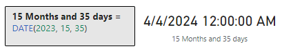
The month argument is a number representing the month, if the value is a number from 1 to 12 then it represents the month of the year (1-January, …, 12-December). However, if the value is greater than 12 a calculation occurs. The date is calculated by adding the value of month to January of the specified year. For example, using DATE if we specify the year as 2023 and the month as 15, we will get a results for March 2024.
15 Months = DATE(2023, 15, 1)

Similarly the argument day is a number representing the day of the month or a calculation. The day argument results in a calculation if the value is greater than the last day of the given month, otherwise it simply represents the day of the month. The calculation is similar to how the month argument works, if day is greater than the last day of the month the value is added to month. If we take the example above and change day to be 35, we can see it returns a date of April 4th, 2024.
DAY, MONTH, YEAR: Extracting Date Components
Sometimes, we just need a piece of the date. Whether it is the day, month, or year, DAX has a function for that. All of these functions have similar syntax and have a singular date argument which can be a date in datetime format or text format (e.g. “2023-01-01”).
DAY(date)
MONTH(date)
YEAR(date)

Note: At the time of writing today is 10/20/2023. The TODAY() function is used through out this post.
These functions are pivotal when segmenting data, creating custom date hierarchies, or performing year-over-year and month-over-month analyses.
TODAY and NOW: Capturing the Present Moment
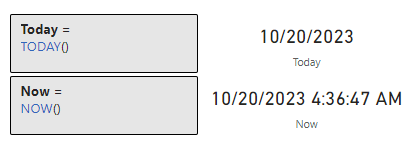
In the dynamic realm of data, real-time insights are invaluable. The TODAY function in DAX delivers the current date without time details. It is perfect for age calculations or determining days since a particular event. Conversely, NOW provides a detailed timestamp, including the current time. This granularity is essential for monitoring live data, event logging, or tracking activities.
The examples above provide examples of using TODAY, the below example highlights the differences between TODAY and NOW.
With these foundational date functions in our tool box we are equipped to continue deeper into DAX’s date and time capabilities. These might seem basic, but their adaptability and functionality are the bedrock for more complex and advanced operations and analyses.
Diving Deeping: Advanced Date Manipulations
As we become more comfortable with DAX’s basic date functions you may begin to wonder what more can DAX’s Date and Time functions do. Diving deeper into DAX’s date functions we will discover more advanced tools specific to addressing date-related challenges. Whether it is shifting dates, pinpointing specific moments, or calculating intervals, DAX’s date and time functions are here to elevate our data analysis and conquer these challenges.
EDATE: Shifting Dates by Month
A common challenge we may encounter is the need to project a date a few months into the future or trace back to a few months prior. EDATE is the function for the job, EDATE allows us to shift a date by a specified number of months. The syntax is:
EDATE(start_date, months)
The start_date is a date in datetime or text format and is the date that we want to shift by the value of months. The months argument is an integer representing the number of months before or after the start_date. One thing to note is that if the start_date is provided in text format the function will interpret this based on the locale and date time settings of the client computer. For example if start_date is 10/1/2023 and the date time settings represent a date as Month/Day/Year this will be interpreted as October 1st, 2023, however if the date time settings represent a date as Day/Month/Year it will be interpreted as January 10th, 2023.
For example, say we follow up on a sale or have a business process that kicks off 3 months following a sale. We can use EDATE to project the SalesDate and identify when this process should occur. We can use:
3 Months after Sale = EDATE(MAX(Sales[SalesDate]), 3)

EOMONTH: Pinpointing the Month’s End
End-of-month dates are crucial for a variety of purposes. With EOMONTH we can easily determine the last date of a month. The syntax is the same as EMONTH:
EOMONTH(start_date, months)
We can use this function to identify the end of the month for each of our sales.
Sales End of Month = EOMONTH(MAX(Sales[SalesDate]), 0)

In the example above we use 0 to indicate we want the end of the month in which the sale occurred. If we needed to project the date to the end of the following month we would update the months argument from 0 to 1.
DATEDIFF & DATEADD: Date Interval Calculations
The temporal aspects of our data can be so much more than static points on a timeline. They can represent intervals, durations, and sequences. By understanding the span between dates or manipulating these intervals we can provide additional insights required by our analysis.
DATEDIFF is the function to use when measuring the span between two dates. With this function we can calculate the age of an item, or the duration of a project. DATEDIFF calculates the difference between the dates base on days, months, or years. Its syntax is:
DATEDIFF(date_1, date_2, interval)
The date_1 and date_2 arguments are the two dates that we want to calculated the difference between. The result will be a positive value if date_2 is larger than date_1, otherwise it will return a negative result. The interval argument is the interval to use when comparing the two dates and can be SECOND, MINUTE, HOUR, DAY, WEEK, MONTH, QUARTER, or YEAR.
We can use DATEDIFF and the following formula to calculate how many days it has been since our last sale, or the difference between our last Sales date and Today.
Days Between Last Sale and Today =
DATEDIFF(MAX(Sales[SalesDate]), TODAY(), DAY)

The above example shows as of 10/20/2023 it has been 64 days since our last sale.
In the DATE: Crafting Dates in Datetime Format section we saw that providing DATE a month value greater than 12 or a day value greater than the last day of the month will add values to the year or month. However, if the goal is to adjust our dates by an specific interval the DATEADD function can be much more useful. Although in the DAX Reference documentation DATEADD is categorized under Time Intelligence functions it is still helpful to mention here. The syntax for DATEADD is:
DATEADD(dates, number_of_intervals, interval)
The dates argument is a column that contains dates. The number_of_intervals is an integer that specifies the number of intervals to add or subtract. If number_of_intervals is positive the calculation will add the intervals to dates and if negative it will subtract the intervals from dates. Lastly, interval is the interval to adjust the dates by and can be day, month, quarter, or year. For more details and examples on DATEADD checkout my previous post Time Travel in Power BI: Mastering Time Intelligence Functions.

Time Travel in Power BI: Mastering Time Intelligence Functions
Journey through the Past, Present, and Future of Your Data with Time Intelligence Functions.
Advanced date manipulations in DAX open up a world of possibilities. From forecasting and backtracking to pinpointing specific intervals. These functions empower us to navigate the intricacies of our data providing clarity and depth to our analysis.
Times Ticking: Harnessing DAX Time Functions
In data analysis, time is so much more than just ticking seconds on a clock. Time provides an element of our data to help understand its patterns looking back, or predicting trends looking forward. DAX provides us a suite of time functions that allow us to dissect, analyze, and manipulate time data.
HOUR, MINUTE, and SECOND: Breaking Down Time Details
Time is a composite of hours, minute, and seconds. DAX provides individual functions that extract each of these components.
As you might have expected these functions are appropriately named HOUR, MINUTE, and SECOND. They also all follow the same general syntax.
HOUR(datetime)
MINUTE(datetime)
SECOND(datetime)
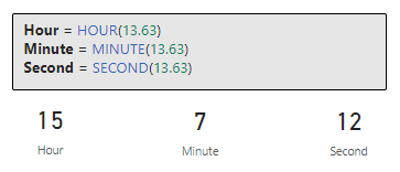
Each function then returns its respective time component, HOUR will return a value from 0 (12:00AM) to 23 (11:00PM), MINUTE returns a value from 0 to 59, and SECOND returns a value also from 0 to 59.
All of these functions take the datetime that contains the component we want to extract as the singular argument. The time can be supplied using datetime format, another expression that returns a datetime (e.g. NOW()), or text in an accepted time format. When the datetime is provided as text the function uses the locale and datetime setting of the client computer to interpret the text value. Most locales use a colon : as the time separator and any text input using colons will parse correctly.

It is also important to be mindful when these functions are provided a numeric value to avoid unintended results. The serial number will first be represented as a datetime data type before the time component is extracted. To more easily understand the results of our calculations its best to first represent these values as datetime data types before passing them to the functions. For example, passing a value of 13.63 to the HOUR function will return a value of 15. This is because 13.63 is first represented as a datetime 1/13/1900 15:07:12 and then the time components are extracted.
TIMEVALUE: Converting Text to Time
In our datasets time values might sometimes be stored as text. The TIMEVALUE function is the go to tool for handling these text values. This function will convert a text representation of time (e.g. "18:15") into a time value. Applying TIMEVALUE converts the text to a time value making it usable for time-based calculations.
Text to Time = TIMEVALUE("18:15")

DAX’s time functions allow us to zero in on the details of our datetime data. When we need to segment data by hours, set benchmarks, or convert time formats, these functions ensure we always have the tools ready to address these challenges.
Special DAX Functions for Date and Time
Dates and times a crucial parts of many analytical tasks. DAX offers a wide array of specialized functions that cater to unique date and time requirements helping us ensure we have the proper tools needed for every analytical challenge we face.
CALENDAR and CALENDARAUTO: Generating a Date Table
When developing our data model having a continuous date table can be an invaluable asset. DAX provides two functions that can help us generate date table within our data model.
CALENDAR will create a table with a single “Date” column containing a contiguous set of dates starting from a specified start date and ending at a specified end date. The syntax is:
CALENDAR(start_date, end_date)
The range of dates is specified by the two arguments and is inclusive of these two dates. CALENDAR will result in an error if start_date is greater than end_date.
CALENDARAUTO takes CALENDAR one step further by adding some automation. This function will generate a date table based on the data already in our data model. It identifies the earliest and latest dates and creates a continuous date table accordingly. When using CALENDARAUTO we do not have to manually specify the start and end date, here is the functions syntax:
CALENDARAUTO([fiscal_year_end_month])
The CALENDARAUTO function has a single optional argument fiscal_year_end_month. This argument can be used to specify the month the year ends and can be a value from 1 to 12. If omitted the default value will be 12.
A few things to note about the automated calculation. The start and end dates are determined by dates in the data model that are not in a calculated column or a calculated table and the function will generate an error if no datetime values are identified in the data model.
NETWORKDAYS: Calculating Workdays Between Two Dates
In business scenarios, understanding workdays is crucial for tasks like planning or financial forecasting. The NETWORKDAYS functions calculates the number of whole workdays between two dates, excluding weekends and providing the options to exclude holidays. The syntax is:
NETWORKDAYS(start_date, end_date[, weekend, holidays])
The start_date and end_date are the dates we want to know how many workdays are between. Within the NETWORKDAYS the start_date can be earlier than, the same as, or later than the end_date. If start_date is greater than end_date the function will return a negative value. The weekend argument is optional and is a weekend number which specifies when the weekends occur, for example a value of 1 (or if omitted) indicates the weekend days are Saturday and Sunday. Check out the parameter details for a list of all the options.
NETWORKDAYS function (DAX) – DAX | Parameters
Learn more about: NETWORKDAYS
Lastly, holidays is a column table of one or more dates that are to be excluded from the working day calendar.
Let’s take a look at an example, from our previous Days Between Last Sale and Today example we know there at 64 days since our last sale. Let’s use the following formula to identify how many of those are workdays.
Workday Between Last Sale and Today =
NETWORKDAYS(MAX(Sales[SalesDate]), [Today], 1)
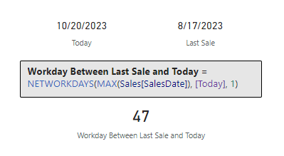
Note: At the time of writing the last sales date is 8/17/2023 and today is 10/20/2023
Taking into account the date range noted above, we can update the Workday Between Last Sale and Today to exclude Labor Day (9/4/2023) using this updated formula.
Workday Between Last Sale and Today (No Holidays) =
NETWORKDAYS(
    MAX(Sales[SalesDate]),
    [Today],
    1,
    {DATE (2023, 9, 4)}
)

QUARTER and WEEKDAY: Understanding Date Hierarchies
When we need to categorized our dates into broader hierarchies functions like QUARTER and WEEKDAY can help with this task. QUARTER returns the quarter of the specified date and returns a number from 1 to 4.
QUARTER(date)

WEEKDAY provides the day number of the week ranging from 1(Sunday) to 7 (Saturday) by default.
WEEKDAY(date, return_type)
The date argument should be in datetime format and entered by using the DATE function or by another expression which returns a date. The return_type determines what value is returned, a value of 1 (or omitted) indicates the week begins on Sunday (1) and ends Saturday (7), 2 indicates the week begins Monday (1) and ends Sunday (7), and 3 the week begins Monday (0) and ends Sunday (6).
Let’s take a look at the WEEKDAY function and return_type by using the following formulas to evaluate Monday, 10/16/2023.
Weekday (1) = WEEKDAY(DATE(2023, 10, 16))
Weekday (2) = WEEKDAY(DATE(2023, 10, 16), 2)
Weekday (3) = WEEKDAY(DATE(2023, 10, 16), 3)

DAX’s specialized date and time functions are helpful tools designed just for us. They cater to the unique requirements of working with date and times, ensuring that we are set to tackle any analytical challenge we may face with precision and efficiency.
Yearly Insights with DAX
The annual cycle holds significance in numerous domains, from finance to academia. Yearly reviews, forecasts, and analyses form the cornerstone of many decision-making processes. DAX offers a set of functions to extract and manipulate year-related data, ensuring you have a comprehensive view of annual trends and patterns.
We have already explored the first function that provides yearly insights, YEAR. This straightforward yet powerful function extracts the year from a given date and allows us to categorize or filter data based on the year. Let’s explore some other DAX functions that help provide us yearly insights into our data.
YEARFRAC: Computing the Year Fraction Between Dates
Sometimes, understanding the fraction of a year between two dates can be beneficial. The YEARFRAC function calculates the fraction of a year between two dates. The syntax is:
YEARFRAC(start_date, end_date[, basis])
Same as other date functions start_date and end_date are the dates we are interested in knowing the fraction of a year between and they are passed to YEARFRAC in datetime format. The basis argument is optional and is the type of day count basis to be used for the calculation. The default value is 0 and indicates the use of US (NASD) 30/360. Other options include 1-actual/actual, 2-actual/360, 3-actual/365, and 4-European 30/360.
Let’s examine the difference between our last sale and today again. From our previous calculation we know there is 64 days between our last sale and today (10/23/2023), we can use YEARFRAC to represent this difference as a fraction of a year.
Fraction of Year Between Last Sale and Today =
YEARFRAC(MAX(Sales[SalesDate]), TODAY(), 0)

WEEKNUM: Determining the Week Number of a Date
Our analysis in many scenarios may require or benefit from understanding weekly cycles. The WEEKNUM function gives us the week number of the specified date, helping us analyze data on a weekly basis. The syntax for WEEKNUM is
WEEKNUM(date[, return_type])
The return_type argument is optional and represents which day the week begins. The default value is 1 indicating the week begins on Sunday.
An important note about WEEKNUM is that the function uses a calendar convention in which the week that contains January 1st is considered to be the first week of the year. However, the ISO 8601 calendar standard defines the first week as the one that has four or more days (contains the first Thursday) in the new year, if this standard should be used the return_type should be set to 21. Check out the Remarks section of the DAX Reference for details on available options.
WEEKNUM function (DAX) – DAX | Remarks
Learn more about: WEEKNUM
Let’s explore the differences between using the default return_type where week one is the week which contains January 1st, and a return_type of 21 where week one is the first week that has four or more days in it (with the week starting on Monday). To do this we will fast forward to Wednesday January 6th, 2027.
In 2027 January 1st lands on a Friday, so using Monday as the start of the week results in 3 days in 2027 being in that week and the first week in 2027 with four or more days (or containing the first Thursday) begins Monday, January 4th.

Harnessing the power of these functions allows us to dive deep into annual trends, make better predictions, and craft strategies that resonate with the yearly ebb and flow of our data.
Wrapping Up Our DAX Temporal Toolkit Journey
Time is a foundational element in data analysis. From understanding past trends to predicting future outcomes, the way we interpret and manipulate time data can significantly influence our insights. DAX offers a robust suite of date and time functions, providing a comprehensive toolkit to navigate the temporal dimensions of our data.
As business continue to trend toward being more data-driven, the need for precise time-based calculations will continue to grow. Whether it is segmenting sales data by quarters, forecasting inventory based on past trends, or understanding productivity across different time zones, DAX provides us the tools to tackle these tasks.
For those looking to continue this journey into DAX and its capabilities there is a wealth of resources available, and a good place to start is the DAX Reference documentation.
Excel Online (Business) – Actions
Learn more about: Power Automate Excel Online (Business) Actions
I have also written about other DAX function groups including Time Intelligence functions, Text Functions, an entire post focused on CALCULATE and an ultimate guide providing a overview of all the DAX function groups.
Time Travel in Power BI: Mastering Time Intelligence Functions
Journey through the Past, Present, and Future of Your Data with Time Intelligence Functions.

Mastering DAX Text Expressions: Making Sense of Your Data One String at a Time
Stringing Along with DAX: Dive Deep into Text Expressions

Unlocking the Secrets of CALCULATE: A Deep Dive into Advanced Data Analysis in Power BI
Demystifying CALCULATE: An exploration of advanced data manipulation.

The DAX Function Universe: A Guide to Navigating the Data Analysis Tool box
Unlock the Full Potential of Your Data with DAX: From Basic Aggregations to Advanced Time Intelligence
In the end, dates are more than just numbers on a calendar and time is more than just ticks on a clock. They are the keys to reveal the story of our data. With the power of DAX Date and Time Functions we will be able to tell this story with ease and in the most compelling way possible.
Thank you for reading! Stay curious, and until next time, happy learning.

And, remember, as Albert Einstein once said, “Anyone who has never made a mistake has never tried anything new.” So, don’t be afraid of making mistakes, practice makes perfect. Continuously experiment and explore new DAX functions, and challenge yourself with real-world data scenarios.
If this sparked your curiosity, keep that spark alive and check back frequently. Better yet, be sure not to miss a post by subscribing! With each new post comes an opportunity to learn something new.


