Discover how to effortlessly navigate through intricate data landscapes using DAX Filter Functions in Power BI.
In the intricate world of Power BI, the ability to skillfully navigate through complex data models is not just a skill, but an art form. This is where DAX Filter Functions come into play, serving as our compass in the often-overwhelming maze of data analysis. These functions give us the power to sift through layers of data with intent and precision, uncovering insights that are pivotal to informed decision-making.
Our journey through data analysis should not be a daunting task. With the right tools and know-how, it can become an adventure in discovering hidden patterns and valuable insights. DAX Filter Functions are the keys to unlocking this information, allowing us to filter, dissect, and examine our data in ways we never thought possible.
Now, let’s embark on a journey to master these powerful functions. Transform our approach to data analysis in Power BI, making it more intuitive, efficient, and insightful. Let DAX Filter Functions guide us through the data maze with ease, leading us to clarity and success in our data analysis endeavors. The path to elevating our Power BI skills starts here, and it starts with mastering DAX Filter Functions.
For those of you eager to start experimenting there is a Power BI report-preloaded with the same data used in this post read for you. So don’t just read, follow along and get hands-on with DAX in Power BI. Get a copy of the sample data file here:

GitHub – Power BI DAX Function Series: Mastering Data Analysis
This dynamic repository is the perfect place to enhance your learning journey.
What are DAX Filter Functions
DAX filter functions are a set of functions in Power BI that allow us to filter data based on specific conditions. These functions help in reducing the number of rows in a table and allows us to focus on specific data for calculations and analysis. By applying well defined filters, we can extract meaningful insights from large datasets and make informed business decisions. Get all the details on DAX Filter Functions here.

Filter Functions (DAX) – Microsoft Learn
Learn more about: Filter functions
In our Power BI report, we can use filter functions in conjunction with other DAX functions that require a table as an argument. By embedding these functions, we can filter data dynamically to ensure our analysis and calculation are using exactly the right data. Let’s dive into some of the commonly used DAX filter functions and explore their syntax and usage.
The ALL Function: Unleashing the Potential of All Our Data
At its core, the ALL function is a powerhouse of simplicity and efficiency. It essentially removes all filters from a column or table, allowing us to view our data in its most unaltered form. This function is our go to tool when we need to clear all filters to create calculation using all the rows in a table The syntax is straightforward:
ALL([table | column[, column[, column[,...]]]])
The arguments to the ALL function must either reference a base table or a base column of the data model, we cannot use table or column expressions with the ALL function. This function serves as a intermediate function that we can use to change the set of results over which a calculation is performed.
ALL can be used in a variety of ways when referencing base tables or columns. Using ALL() will remove filters everywhere and can only be used to clear filters but does not return a table. When referencing a table, ALL(<table>), the function removes all the filters from the specified table and returns all the values in the table. Similarly, when referencing columns, ALL([, [, ...]]), the function removes all filters from the specified column(s) in the table, while all other filters on other column in the table still apply. When referencing columns, all the column argument must come from the same table.
While, we can use ALL to remove all context filters from specified columns, there is another function that can be helpful. ALLEXCEPT is a DAX function that removes all context filters in the table except filters that have been applied to the specified columns. For more details check out the Microsoft documentation on ALLEXCEPT.

Learn more about: ALLEXCEPT
Practical Examples: Navigating Data with the ALL Function
Considering the dataset in our sample report, suppose we want to analyze the overall sales performance, irrespective of any specific regions or dates. Using the following formula, we can provide the total sales amount across all regions and times by removing any existing filters on the Sales table.
All Sales =
SUMX(
   ALL(Sales),
   Sales[Amount]
)
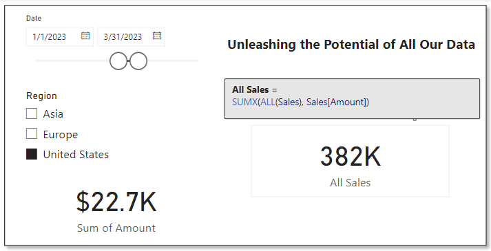
In the above example we can see the card visual on the bottom left is the default sum aggregation of the Amount column in our sales table. Specifically, with the slicers on the report, this card shows the total sales within the United States region during the period between 1/1/2023 and 3/31/2023. We can use the ALL function to display to total sales amount across all regions and irrespective of time, shown on the card visual on the right.
This functionality is particularly useful when making comparative analyses. For instance, we could use this to determine a region’s contribution to total sales. We can compare the sales in a specific region (with filters applied) to the overall sales calculated using ALL. This comparison offers valuable insights into the performance of different segments relative to the total context.

ALLSELECTED Decoded: Interactive Reporting’s Best Friend
The ALLSELECTED function in DAX takes the capabilities of ALL a step further. It is particularly useful in interactive reports where our users apply filters. This function respects the filters applied by our report users but disregards any filter context imposed by report objects like visuals or calculations. The syntax is:
ALLSELECTED([tableName | columnName[, columnName[, columnName[,…]]]] )
Similar to ALL the tableName and columnName parameters are optional and reference an existing table or column, an expression cannot be used. When we provide ALLSELECTED a single argument it can either be tableName or columnName, and when we provide the function more than one argument, they must be columns from the same table.
ALLSELECTED differs from ALL because it retains all filters explicitly set within the query, and it retains all context filters other than row and column filters.
Practical Examples: Exploring ALLSELECTED and How it Differs From ALL
At first glance it may seem as if ALL and ALLSELECTED perform the same task. Although, these two functions are similar there is an important difference between them. ALLSELECTED will ignore filters applied by report visuals, while ALL will ignore any filters applied within the report. Let’s explore this difference with an example.
We will use three measures to explore ALLSELECTED. First a measure that simply calculates the sum of our Sales Amount, here is its definition.
Total Sales = SUM(Sales[Amount])
Second a measure using the function explored in the previous section ALL.
Sales ALL = CALCULATE(
    SUM(Sales[Amount]),
    ALL(Sales)
)
Lastly, a measure that uses ALLSELECTED.
Sales ALLSELECTED =
CALCULATE(
    SUM(Sales[Amount]),
    ALLSELECTED(Sales)
)
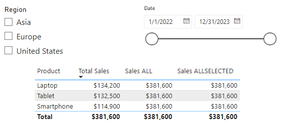
After creating the measures, we can add a table visual including the Product field and these three measures. When the report has no filters due to interacting with the slicers on the report, we can see that the Total Sales measure gets filtered by the Product column and shows the total sales for each product. However, the other two measure show the overall total sales.
The inclusion of the Product column in the table visual is filtering the values and impacting the calculation of the Total Sales measure, while the other two measure are using all of the sales records in their calculation.
Next let’s use the Region and Date slicers to explore the differences between ALL and ALLSELECTED. As expected, all the additional filtering due to the slicer selections continues to impact our Total Sales measure.
Additionally, we see the ALLSELECTED measure gets filtered based on the external slicer selections but continues to not be impacted by the internal filtering of the table visual. This differs from our measure that uses the ALL function, which continues to show the grand total sales value. This is because the ALL function ignores any filter implicit from the visual or explicit from external slicers.
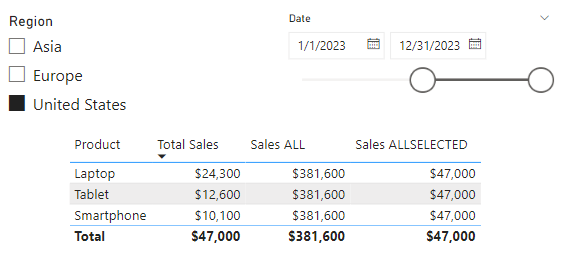
The difference between ALL and ALLSELECTED boils down to ALL will ignore any filter applied, while ALLSELECTED will ignore just the filter applied by the visual.
The necessity of ALLSELECTED is its ability to respect user’s interactions and filtering choices on slicers or other interactive elements. Unlike ALL, which disregards all filters, ALLSELECTED maintains the interactive nature or our reports, ensuring that the calculations dynamically adapt to user inputs.
So, what is a use case for ALLSELECTED? A common use is calculating percentages, based on a total value that is dependent on user interaction with report slicers. Check out this post, on how this function can be used along with ISINSCOPE to calculate context aware insights.

ISINSCOPE: The Key to Dynamic Data Drilldowns
Elevate Your Power BI Report with Context-Aware Insights
CALCULATE: The Engine for Transforming Data Dynamically
CALCULATE is one of the most versatile and powerful functions in DAX, acting as a cornerstone for many complex data operations in Power BI. It allows us to manipulate the filter context of a calculation, letting us perform dynamic and complex calculations with ease. CALCULATE follows a simple structure.
CALCULATE(expression[, filter1[, filter2[, …]]])
The expression parameter is the calculation we want to perform, and the filter parameters are optional boolean expressions or table expression that define our filters or filter modifier functions. Boolean filter expressions are expressions that evaluate to true or false, and when used with CALCULATE there are certain rules that must be followed, see the link below for details. Table filter expressions apply to a table, and we can use the FILTER function to apply more complex filtering conditions, such as those that cannot be defined by using a boolean filter expression. Finally, filter modifier functions provide us even more control when modifying the filter context within the CALCULATE function. Filter modifier functions include functions such as REMOVEFILTERS, KEEPFILTERS, and the ALL function discussed in the previous section.
Find all the required details in the documentation.

CALCULATE Function (DAX) – Parameters
Learn more about: CALCULATE
Practical Examples: Using CALCULATE for Dynamic Data Analysis
Let’s say that for our report we are required to calculate the total sales in the United States region. We can use CALCULATE and this expression to meet this requirement.
United States Sales =
CALCULATE(
   SUM(Sales[Amount]),
   Regions[Region]="United States"
)
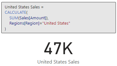
We can continue to build on the previous example to further examine sales in the United States. For this example, we will compare the average sales of smartphones in the United States against the benchmark of average sales of smartphones across all regions.
US Smartphone Sales vs. Average Smartphone Sales =
    CALCULATE(
        AVERAGE(Sales[Amount]),
        Products[Product] = "Smartphone",
        Regions[Region] = "United States"
    )
    - AVERAGEX(
        FILTER(
            Sales,
            RELATED(Products[Product]) = "Smartphone"
        ),
        Sales[Amount]
)

These two examples just begin to scratch the surface of what is possible when we utilize the CALCULATE function. For more examples and more details on CALCULATE check out this post that provides a deep dive into the CALCULATE function.

Unlocking the Secrets of CALCULATE: A Deep Dive into Advanced Data Analysis in Power BI
Demystifying CALCULATE: An exploration of advanced data manipulation.
CALCULATE proves indispensable for redefining the filter context impacting our calculations. It empowers us to perform targeted analysis that goes beyond the standard filter constraints of a report, making it an essential tool in our DAX toolbox.
Mastering FILTER: The Art of Precision in Data Selection
The FILTER function in DAX is a precision tool for refining data selection within Power BI. It allows us to apply specific conditions to a table or column, creating a subset of data that meets the criteria. The FILTER function returns a table that represents a subset of another table or expression, and the syntax is as follows.
FILTER(table, filter)
The table argument is the table, or an expression that results in a table, that we want to apply the filter to. The filter argument is a boolean expression that should be evaluated for each row of the table.
FILTER is used to limit the number of rows in a table allowing for us to create specific and precise calculations. When we use the FILTER function we embed it within other functions, we typically do not use it independently.
When developing our Power BI reports a common requirement is to develop DAX expressions that need to be evaluated within a modified filter context. As we saw in the previous section CALCULATE is a helpful function to modify the filter context, and accepts filter arguments as either boolean expressions, table expression or filter modification functions. Meaning CALCULATE, will accept the table returned by FILTER as one of its filtering parameters, however it is generally best practice to avoid using the FILTER function as a filter argument when a boolean expression can be used. The FILTER function should be used when the filter criteria cannot be achieved with a boolean expression. Here is an article that details this recommended best practice.

Avoid using FILTER as a Filter Argument
Best practices for using the FILTER function as a filter argument.
For example, we have two measures below that calculate the total sales amount for the United States. Both of these measures correctly filter our data and calculate the same value for the total sales. When possible, the best practice is to use the expression on the left which passes the filter arguments to CALCULATE as a boolean expression. This is because when working with Import model tables that are store in-memory column stores, they are explicitly optimized to filter column in this way.

Practical Examples: FILTER Functions Illustrated
Let’s now see how FILTER can help us build on our analysis of US Smartphone Sales. In the previous section we created a US Smartphone Sales vs Average Smartphone Sales measure to visualize US sales against a benchmark. Now we are interested in the total sales amount for each quarter that average US smartphones sales is below the benchmark. FILTER can help us do this with the following expression.
United States Sales FILTER =
   CALCULATE(
      SUM(Sales[Amount]),
      FILTER(
         VALUES(DateTable[YearQuarter]),
         [US Smartphone Sales vs. Average Smartphone Sales] < 0
      )
   )

FILTER is particularly useful when we require a detailed and specific data subset. It is a function that brings granular control to our data analysis, allowing for a deeper and more focused exploration of our data.
Dynamic Table Creation with CALCULATETABLE
The CALCULATETABLE function in DAX is a powerful tool for creating dynamic tables based on specific conditions. This function performs provides us the same functionality that CALCULATE provides, however rather than returning a singular scalar value CALCULATETABLE returns a table. Here is the function’s syntax:
CALCULATETABLE(expression[, filter1[, filter2[, …]]])
This may look familiar, CALCULATETABLE has the same structure as CALCULATE for details on the expression and filter arguments check out the previous section focused on the CALCULATE function.
Practical Examples: Apply CALCULATETABLE
Let’s say we want to calculate the total sales for the current year so we can readily visualize the current year’s sale broken down by product, region and employee. CALCULATETABLE can help us achieve this with the following expression.
Current Year Total Sales =
SUMX(
   CALCULATETABLE(
      Sales,
      YEAR(Sales[SalesDate]) = YEAR(TODAY())
   ),
   Sales[Amount]
)

CALCULATETABLE proves to be invaluable when we need to work with a subset of data based on dynamic conditions. It’s flexibility to reshape our data on the fly makes it an essential function for nuanced and specific data explorations in Power BI.
Resetting the Scene with REMOVEFILTERS
The REMOVEFILTERS function in DAX is crucial for when we need to reset or remove specific filters applied to our data. It allows for recalibration of the filter context, either entirely or partially. The syntax for this function is:
REMOVEFILTERS([table | column[, column[, column[,…]]]])
Looking at the structure of REMOVEFILTERS, we can see it is similar to that of ALL and ALLSELECTED. Although these functions are similar it is important to differentiate them. While ALL removes all filters from a column or table and ALLSELECTED respects user-applied filter but ignores other filter contexts, REMOVEFILTERS specifically targets and removes filters from the specified columns or tables, offering us more control and precision.
Practical Examples: Implementing REMOVEFILTERS
Let’s start by adding a new measure to our previous table visual where we explored the difference between ALL and ALLSELECTED to highlight the difference between these functions.
We will create a new measure and add it to the table visual, the new measure is:
Sales REMOVEFILTER Region =
CALCULATE(
   SUM(Sales[Amount]),
   REMOVEFILTERS(Regions[Region])
)
This expression will calculate the total sales disregarding any Region filter that might be in place.

Here we can see this new Sales REMOVEFILTER Region measure shows the total sales respecting the row context of Product on the table visual and the selected dates on the date slicer, however, removes the Region filter that would apply due to the Region slicer.
Let’s take a look at how we can apply and leverage the differences between these functions. We can use our Total Sales and the other three measures to calculate various percentages to provide additional insights.
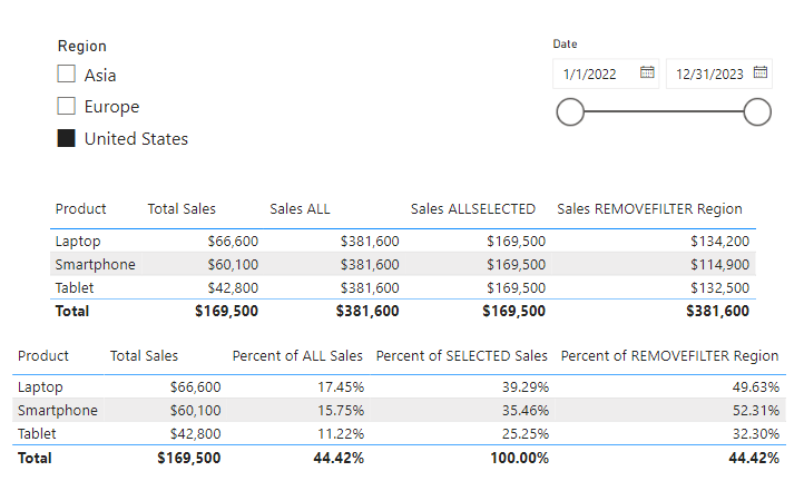
REMOVEFILTERS offers a tailored approach to filter removal, differing from ALL which disregards all filters unconditionally, and ALLSELECTED which adapts to user selections. This makes REMOVEFILTERS an essential function for creating more nuanced and specific measures in our Power BI reports.
LOOKUPVALUE: Bridging Tables in Analysis
The LOOKUPVALUE function in DAX is a powerful feature for cross-referencing data between tables. It allows us to find a value in a table based on matching a value in another table or column.
LOOKUPVALUE (
    result_columnName,
    search_columnName,
    search_value
    [, search2_columnName, search2_value]…
    [, alternateResult]
)
Here result_columnName is the name of an existing column that contains the value we want to be returned by the function; it cannot be an expression. The search_columnName argument is the name of an existing column and can be in the same table as the result_columnName or in a related table, the search_value is the value to search for within the search_columnName. Finally, the alternativeResult is an optional argument that will be returned when the context for result_columnName has been filter down to zero or more than one district value, when not specified LOOKUPVALUE will return BLANK.
LOOKUPVALUE is essential for scenarios where data relationships are not directly defined through relationships in the data model. If there is a relationship between the table that contains the result column and tables that contain the search column, typically using the RELATED function rather than LOOKUPVALUE is more efficient.
Practical Examples: LOOKUPVALUES Explored
Let’s use LOOKUPVALUE to connect sales data with the respective sales managers. We need to identify the manager for each sale in our Sales table for our report. We can use a formula that first finds the manager’s ID related to each sale. For details on how we can user Parent and Child Functions to work with hierarchical data check out the Parent and Child Functions: Managing Hierarchical Data section of this post.

The DAX Function Universe: A Guide to Navigating the Data Analysis Tool box
Unlock the Full Potential of Your Data with DAX: From Basic Aggregations to Advanced Time Intelligence
In the example in the post above we use PATH and PATHITMEREVERSE to navigate the organizational hierarchy to identify the manager’s ID of each employee. Then utilizing REALTED and LOOKUPVALUE we can add a new calculated column to our Sales table listing the Sales Manager for each sale. We can use the following formula that first finds the manager’s ID related to each sale and then fetches the manager’s name using the LOOKUPVALUE function.
Sales Manager Name =
VAR ManagerID = RELATED(Employee[ManagerID])

RETURN
LOOKUPVALUE(Employee[EmployeeName], Employee[EmployeeID], ManagerID)

In this example, the RELATED function retrieves the ManagerID for each sale from the Employees table. Then, LOOKUPVALUE is used to find the corresponding EmployeeName (the manager’s name) in the same table based on the ManagerID. This approach is particulariy beneficial in scenarios where understanding hierarchical relationships or indirect associations between data points is crucial.
By using LOOKUPVALUE in this manner, we add significant value to our reports, offering insights into the managerial oversight of sales activities, which can be pivotal for performance analysis and strategic planning.
Mastering DAX Filter Functions for Advanced Analysis
Now that we have finished our exploration of DAX Filter Functions in Power BI, it is clear that these tools are not just functions, they are the building blocks for sophisticated data analysis. From the comprehensive clearing of contexts with ALL to dynamic and context-sensitive capabilities of CALCULATE and FILTER, each function offers a unique approach to data manipulation and analysis.
Understanding and applying functions like ALLSELECTED, REMOVEFILTERS and LOOKUPVALUE enable us to create reports that are not only insightful but also interactive and responsive to user inputs. They allow use to navigate through complex data relationships with ease, bringing clarity and depth to our analyses.
As we continue our journey in data analytics, remember that mastering these functions can significantly enhance our ability to derive meaningful insights from our data. Each function has its place and purpose, and knowing when and how to use them will set us apart as proficient Power BI analyst.
Embrace these functions as we delve deeper into our data and watch as they transform our approach to business intelligence and data storytelling. Happy analyzing!
Thank you for reading! Stay curious, and until next time, happy learning.
And, remember, as Albert Einstein once said, “Anyone who has never made a mistake has never tried anything new.” So, don’t be afraid of making mistakes, practice makes perfect. Continuously experiment and explore new DAX functions, and challenge yourself with real-world data scenarios.
If this sparked your curiosity, keep that spark alive and check back frequently. Better yet, be sure not to miss a post by subscribing! With each new post comes an opportunity to learn something new.


