Elevate Your Productivity with Planner and Power Automate

November 22, 2023November 22, 2023emguyant Leave a comment

Unlock the secrets to enhanced productivity and seamless project management.

Introduction to Power Automate and Microsoft Planner

In today’s fast-paced business environment, mastering the art of productivity is not just an option, but a necessity. The dynamic duo of Microsoft Planner and Power Automate are our allies in the realm of project and task management. Imagine a world where our projects flow seamlessly, where every task aligns perfectly with your goals, and efficiency is not just a buzzword but a daily reality. This is all achievable with the integrations of Microsoft Planner and Power Automate in your corner.

Microsoft Planner, is our go-to task management tool, that allows us and our teams to effortlessly create, assign, and monitor tasks. It provides a central hub where tasks aren’t just written down but are actively managed and collaborated on. Its strength lies in its visual organization of tasks, with dashboard and progress indicators providing an bird’s-eye view of our project, making organization and prioritization a breeze. It is about managing the chaos of to-dos into an organized methodology of productivity, with each task moving smoothly from To Do to Done.

On the other side of this partnership we have Power Automate, the powerhouse of process automation. It bridges the gap between our various applications and services, automating the mundane so we can focus on what is important. Power Automate is our behind the scenes tool for productivity, connecting our favorite apps and automating workflows whether that’s collecting data, managing notifications, sending approvals, and so much more all without us lifting a finger, after the initial setup of course.

Together, these tools don’t just manage tasks; they redefine the way we approach project management. They promise a future where deadlines are met with ease, collaboration is effortless, and productivity peaks are the norm.

Ready to transform your workday and elevate your productivity? Let Microsoft Planner and Power Automate streamline your task management.

Here’s an overview of what is explored within this post. Start with an overview of Power Automate triggers and actions specific to Microsoft Planner or jump right to some example workflows.

Unveiling the Power of Planner Triggers in Power Automate

Exploring Planner triggers in Power Automate reveals a world of automation that streamlines task management and enhances productivity. Let’s dive into three key triggers and their functionalities.

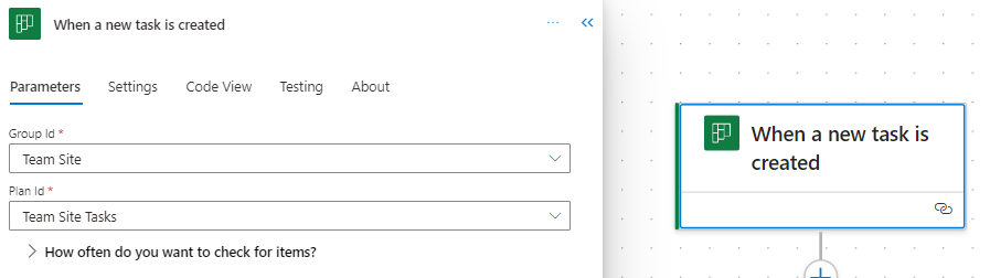
When a new task is created

This trigger jumps into action as soon as a new task is created in Planner. It requires the Group Id and Plan Id to target the specific Planner board. This trigger can set a series of automated actions into motion, such as sending notifications to relevant team members, logging the task in an Excel reporting workbook, or triggering parallel tasks in a related project.

When a task is assigned to me

This trigger personalizes your task management experience. It activates when a task in Planner is assigned to you. This trigger can automate personal notifications, update your calendar with the new tasks, or prepare necessary documents or templates associated with the task. Simply select this Planner trigger and it is all set, there is no additional information required by the trigger. It’s an excellent way to stay on top of personal responsibilities and manage your workload efficiently.

When a task is completed

The completion of a task in Planner can signal the start of various subsequent actions, hinging on the completion status of a task in a specified plan. The required inputs are the Group Id and the Plan Id to identify the target Planner board. This trigger is instrumental in automating post-task processes like updating project status reports, notifying team members or stakeholders of the task completion, or archiving task details for accountability and future reference.

By leveraging these Planner triggers in Power Automate, we can not only automate but also streamline our workflows. Each trigger offers a unique avenue to enhance productivity and ensures that our focus remains on strategic and high-value tasks.

Navigating Planner Actions in Power Automate

Navigating the complexities of project management requires tools that offer both flexibility and control. The integration of Microsoft Planner actions within Power Automate provides a robust solution for managing tasks efficiently. By leveraging Planner actions in Power Automate, we can automate and refine our task management processes. Let’s dive into some of the different Planner actions.

Adding and Removing assignees

Task assignment is a critical aspect of project management. These actions in Power Automate facilitate flexible and dynamic assignment and reassignment of team members to tasks in Planner, adapting to the ever-changing project landscape.

Add assignees to a task
This action allows us to assign team members to specific tasks, with inputs including the task ID and the user ID(s) of the assignee(s). It’s particularly useful for quickly adapting to changes in project scope or team availability, ensuring that tasks are always in the right hands.

Remove assignees from a task
Inputs for this action are the task ID and the user ID(s) of the assignee(s) to be removed. It’s essential for reorganizing task assignments when priorities shift or when team members need to be reallocated to different tasks, maintaining optimal efficiency.

Creating and Deleting tasks

The lifecycle of a task within any project involves its creation and eventual completion or removal. These actions in Power Automate streamline these essential stages, ensuring seamless task management within Planner.

Create a task
Every project begins with a single step, or in the case of our Planner board, a single task. To create a task we must provide the essentials, including Group Id, Plan Id, and Title. This action is invaluable for initiating tasks in response to various Power Automate triggers, such as email requests or meeting outcomes, ensuring timely task setup.

When using the new Power Automate designer (pictured above), be sure to provide all optional details of the task by exploring the Advanced parameters dropdown. Under the advanced parameters we will find task details to set in order to create a task specific to what our project requires. We can set the newly created task’s Bucket Id, Start Date Time, Due Date Time, Assigned User Id, as well as applying any tags needed to create a detailed and well defined task. When using the classic designer we will see all these options listed within the action block.

Delete a task
Keeping our Planner task list updated and relevant is equally important to successful project lifecycle management. Removing completed, outdated, or irrelevant tasks can help us maintain clarity and focus on the overall project plan. This action just requires us to provide the Task Id of the task we want deleted from our Planner board.

Getting and Updating tasks

Accessing and updating task information are key aspects of maintaining project momentum. These actions provide the means to efficiently manage task within Planner.

Get a task
Understanding each task’s status is crucial for effective management, and the Get a task action offers a window into the life of any task in our Planner board. By providing the Task Id, this action fetches the task returning information about the specific task. It is vital for our workflows that require current information about a task’s status, priority, assignees, or other details before proceeding to subsequent steps. This insight is invaluable for keeping a pulse on our projects progress.

Update a task
This action, requires the Task Id and the task properties to be updated, allowing for real-time modifications of task properties. It is key for adapting tasks to new deadlines, changing assignees, or updating a task’s progress. Using this action we can ensure that our Planner board always reflects the most current state of our tasks providing a current overview of the overall project status.

Getting and Updating task details

Detailed task management is often necessary for complex projects. These actions cater to this need by providing and updating in-depth information about tasks in Planner.

Get task details
Each task in a project has its own story, filled with specific details and nuances. This action offers a comprehensive view of a task, including its description, checklist items, and more. It is an essential action for workflows that require a deep understanding of task specifics for reporting, analysis, or decision making.

Update task details
With inputs for detailed aspects of our tasks, such as its descriptions and checklist items, this action allows for precise and thorough updates to our task information. It is particularly useful for keeping tasks fully aligned with project developments and team discussions.

List buckets

Effective task categorization is vital for clear project visualization and management. The List buckets action in Power Automate is designed to provide a comprehensive overview of task categories or buckets within our Planner board. We provide this action the Group Id and Plan Id and it returns a list of all the buckets within the specified plan, including details like bucket Id, name, and an order hint.

This information can aid in our subsequent actions, such as creating a new task within a specific bucket on our Planner board.

List Tasks

Keeping a tab on all tasks within a project is essential for effective project tracking, reporting, and management. The List tasks action in Power Automate offers a detailed view of tasks within a specific planner board.

We need to provide this action the Group Id and Plan Id, and it provides a detailed list of all tasks. The details provided for each task include the title, start date, due date, status, priority, how many active checklist items the task has, categories applied to the task, who created the task, and who the task is assigned to. This functionality is invaluable for teams to gain insights into task distribution, progress, and pending actions, ensuring that no task is overlooked and that project milestones are met.

Basic Workflows: Simplifying Task Management with Planner and Power Automate

Before diving into some more advanced examples and integrations, it is essential to understand how Planner and Power Automate can simplify everyday task management through some basic workflows. These workflows will provide a glimpse into the potential of combining these two powerful tools.

Weekly Summary of Completed Tasks

This workflow automates the process of summarizing completed tasks in Planner, sending a weekly email to project managers so they can keep their finger on the pulse of project progress.

The flow has a reoccurrence trigger which is set to run the workflow on a weekly basis. The workflow then starts by gathering all the tasks from the planner board using the List tasks action. This action provides two helpful task properties that we can use to pinpoint the task that have been completed in the last week.

The first is percentComplete, we add a filter data operation action to our workflow and filter to only tasks that have a percentComplete equal to 100 (i.e. are marked completed). We set the From input to the value output of the List task action and define our Filter Query.

The second property we can use from List tasks is the completedDateTime, we can use this to further filter our completed task to just those completed within the last week. Here we use the body of our Filter array: Completed tasks action and use an expression to calculated the difference between when the task was completed and when the flow is ran, in days.

The expression used in the filter query is:

int(split(dateDifference(startOfDay(getPastTime(1, 'Week')), item()?['completedDateTime']), '.')[0])

This expression starts by getting the start of the day 1 week ago using getPastTime and startOfDay. Then we calculate the difference using dateDifference. The date difference function will return a string value in the form of 7.00:00:00.0000000, representing Days.Hours:Minutes:Seconds. For our purposes we are only interested in the number of days, specifically whether the value is positive or negative, that is was it completed before or after the date 1 week ago. To extract just the days as an integer we first use split to split the string based on periods, and then we use the first item in the resulting array ([0]), and pass this to the int function, to get a final integer value.

We then use the Create HTML table action to create a summary table of the Planner tasks that were completed in the past week.

Then we can send out an email to those that require the weekly summary of completed tasks, using the output of the Create HTML table: Create summary table action.

Here is an overview of the entire Power Automate workflow that automates our process of summarizing our Planner tasks that have been completed in the past week.

This automated summary is invaluable for keeping track of progress and upcoming responsibilities, ensuring that our team is always aligned and informed about the week’s achievements and ready to plan for what is next.

Post a Teams message for Completed High Priority Tasks

This workflow is tailored to enhance team awareness and acknowledgement of completed high-priority tasks. It automatically sends a Teams notification when a high-priority task in Planner is marked as completed.

The workflow triggers when a Planner task on the specified board is marked complete. The workflow then examines the priority property of the task to determine if a notification should be sent. For the workflow a high-priority task is categorized as a task marked as Important or Urgent in Planner.

The workflow uses a condition flow control to evaluate each task’s priority property. An important note here is that, although in Planner the priorities are shown as Low, Medium, Important, and Urgent, the property values associated with these values are stored in the task property as 9, 5, 3, 1, respectively. So the condition used evaluates to true if the priority value is less than or equal to 3, that is the task is Important or Urgent.

When the condition is true, the workflow gathers more details about the task and then sends a notification to keep the team informed about these critical tasks.

Let’s break down the three actions used to compose and send the Teams notification. First, we use the List buckets action to provide a list of all the buckets contained within our Planner board. We need this to get the user friendly bucket name, because the task item only provides us the bucket id.

Then we can use use the Filter data operation to filter the list of all the buckets to the specific bucket the complete task resides in.

Here, value is the output of our List bucket action, id is the current bucket list item, and bucketId is the id of the current task item of the For each: Completed task loop. We can then use the dynamic content from the output of this action to provide a bit more detail to our Teams notification.

Now we can piece together helpful information and notify our team when high-priority tasks are completed using the Teams Post a message in a chat or channel action, shown above. Providing our team details like the task name, the bucket name, and a link to the Planner board.

These basic yet impactful workflows illustrate the seamless integration of Planner with Power Automate, setting the stage for more advanced and interconnected workflows. They highlight how simple automations can significantly enhance productivity and team communication.

Advanced Workflows: Leveraging Planner with Excel and GitHub Integrations

The integration of Microsoft Planner with other services through Power Automate unlocks new dimensions in project management, offering innovative ways to manage tasks and enhance collaboration.

Excel Integration for Reporting Planner Tasks

A standout application of this integration is the reporting of Planner tasks in Excel. By establishing a flow in Power Automate, task updates from Planner can be seamlessly merged to an Excel workbook. This setup is invaluable for generating detailed reports, tracking project progress, and providing more in-depth insights.

For an in-depth walkthrough of a workflow, leveraging this integration check out this post that covers the specifics of setting up and utilizing this integration.

Transforming Project Tracking: How to Merge Planner with Excel Using Power Automate

Explore the Detailed Workflow for Seamless Task Management and Enhanced Reporting Capabilities.

GitHub Integration for Automated Task Creation

Combining Planner with GitHub through Power Automate creates a streamlined process for managing software development tasks. A key workflow in this integration is the generation of Planner tasks in response to new GitHub issues assigned to you. When an issue is reported in GitHub, a corresponding task is automatically created in Planner, complete with essential details from the GitHub issue. This integration ensures prompt attention to issues and their incorporation into the broader project management plan.

Check back, for a follow up post focus specifically on providing a detailed guide on implementing this workflow.

These advanced workflows exemplify the power and flexibility of integrating Planner with other services. By automating interactions across different platforms, teams can achieve greater efficiency and synergy in their project management practices.

Unleashing New Dimensions in Project Management with Planner and Power Automate

Finishing our exploration of Microsoft Planner and Power Automate, it’s evident that these tools are more than mere facilitators of task management and workflow automation. They embody a transformative approach to project management, blending efficiency, collaboration, and innovation in a unique and powerful way.

The synergy between Planner and Power Automate opens up a realm of possibilities, enabling teams and individuals to streamline their workflows, integrate with a variety of services, and automate processes in ways that were previously unimaginable. From basic task management to complex, cross-platform integrations with services like Excel and GitHub, these tools offer a comprehensive solution to the challenges of modern project management.

The journey through the functionalities of Planner and Power Automate is a testament to the ever-evolving landscape of digital tools and their impact on our work lives. As these tools continue to evolve, they offer fresh opportunities for enhancing productivity, fostering team collaboration, and driving innovative project management strategies.

Experiment with these tools and explore the myriad of features they have to offer, and discover new ways to optimize your workflows. The combination of Planner and Power Automate isn’t just a method for managing tasks; it’s a pathway to redefining project management in the digital age, empowering teams to achieve greater success and efficiency.

Thank you for reading! Stay curious, and until next time, happy learning.

And, remember, as Albert Einstein once said, “Anyone who has never made a mistake has never tried anything new.” So, don’t be afraid of making mistakes, practice makes perfect. Continuously experiment, explore, and challenge yourself with real-world scenarios.

If this sparked your curiosity, keep that spark alive and check back frequently. Better yet, be sure not to miss a post by subscribing! With each new post comes an opportunity to learn something new.

Temporal Triumphs with DAX Date and Time Functions

October 20, 2023March 26, 2024emguyant Leave a comment

Explore the ebb and flow of the temporal dimension of your data with DAX’s suite of Date and Time Functions.

In data analysis, understanding the nuances of time can be the difference between a good analysis and a great one. Time-based data, with its intricate patterns and sequences offers a unique perspective into trends, behaviors, and potential future outcomes. DAX provides specialized date and time functions helping guide us through the complexities of temporal data with ease.

Curious what this post will cover? Here is the break down, read top to bottom or jump right to the part you are most interested in.

For those of you eager to start experimenting there is a Power BI report pre-loaded with the sample data used in this post ready for you. So don’t just read, following along and get hands-on with DAX in Power BI. Get a copy of sample data file (power-bi-sample-data.pbix) here:

GitHub – Power BI DAX Function Series: Mastering Data Analysis

This dynamic repository is the perfect place to enhance your learning journey and serves as an interactive compliment to the blog posts on EthanGuyant.com.

The Power of Date and Time in Data Analysis

Consider the role of a sales manager for a electronic store. Knowing 1,000 smartphones were sold last month provides a good snapshot. But, understanding the distribution of these sales-like the surge during weekends or the lull on weekdays-offers greater insights. This level of detail is made possible by time-based data and allows for more informed decisions and strategies.

DAX and Excel: Spotting the Differences

For many, the journey into DAX begins with a foundation in Excel and the formulas it provides. While DAX and Excel share a common lineage, they two have distinct personalities and strengths. Throughout this post if you are familiar with Excel you may recognize some functions but it is important to note that Excel and DAX work with dates differently.

Both DAX and Excel boast a rich array of functions, many of which sound and look familiar. For instance the TODAY() function exists in both. In Excel, TODAY() simply returns the current date. In DAX, while TODAY() also returns the current date it does so within the context of the underlying data model, allowing for more complex interactions and relationships with other data in Power BI.

Excel sees dates and times as serial numbers, a legacy of its spreadsheet origins. DAX, on the other hand, elevates them with a datetime data type. This distinction means that in DAX, dates and times are not just values, they are entities with relationships, hierarchies, and attributes. This depth allows for a range of calculations in DAX that would require workarounds in Excel. And with DAX’s expansive library of date time functions, the possibilities are vast.

For more details on DAX date and time functions keep reading and don’t forget to also checkout the Microsoft documentation.

Date and Time Functions

Learn more about: Date and time functions

Starting Simple: Basic Date Functions in DAX

Diving into DAX can fell like like stepping into the ocean. But fear not! Let’s wade into the shallows first by getting familiar with some basic functions. These foundational functions will set the stage for more advanced explorations later on.

DATE: Crafting Dates in Datetime Formats

The DATE function in DAX is a tool for manually creating dates. It syntax is:

DATE(year, month, day)

As you might expect, year is a number representing the year. What may not be as clear is the year argument can include one to four digits. Although years can be specified with two digits it best practice to use four digits whenever possible to avoid unintended results. For example:

Use Four Digit Years = DATE(23, 1, 1)

Will return January 1st, 1923, not January 1st, 2023 as may have been intended.

The month argument is a number representing the month, if the value is a number from 1 to 12 then it represents the month of the year (1-January, …, 12-December). However, if the value is greater than 12 a calculation occurs. The date is calculated by adding the value of month to January of the specified year. For example, using DATE if we specify the year as 2023 and the month as 15, we will get a results for March 2024.

15 Months = DATE(2023, 15, 1)

Similarly the argument day is a number representing the day of the month or a calculation. The day argument results in a calculation if the value is greater than the last day of the given month, otherwise it simply represents the day of the month. The calculation is similar to how the month argument works, if day is greater than the last day of the month the value is added to month. If we take the example above and change day to be 35, we can see it returns a date of April 4th, 2024.

DAY, MONTH, YEAR: Extracting Date Components

Sometimes, we just need a piece of the date. Whether it is the day, month, or year, DAX has a function for that. All of these functions have similar syntax and have a singular date argument which can be a date in datetime format or text format (e.g. “2023-01-01”).

DAY(date)
MONTH(date)
YEAR(date)

Note: At the time of writing today is 10/20/2023. The TODAY() function is used through out this post.

These functions are pivotal when segmenting data, creating custom date hierarchies, or performing year-over-year and month-over-month analyses.

TODAY and NOW: Capturing the Present Moment

In the dynamic realm of data, real-time insights are invaluable. The TODAY function in DAX delivers the current date without time details. It is perfect for age calculations or determining days since a particular event. Conversely, NOW provides a detailed timestamp, including the current time. This granularity is essential for monitoring live data, event logging, or tracking activities.

The examples above provide examples of using TODAY, the below example highlights the differences between TODAY and NOW.

With these foundational date functions in our tool box we are equipped to continue deeper into DAX’s date and time capabilities. These might seem basic, but their adaptability and functionality are the bedrock for more complex and advanced operations and analyses.

Diving Deeping: Advanced Date Manipulations

As we become more comfortable with DAX’s basic date functions you may begin to wonder what more can DAX’s Date and Time functions do. Diving deeper into DAX’s date functions we will discover more advanced tools specific to addressing date-related challenges. Whether it is shifting dates, pinpointing specific moments, or calculating intervals, DAX’s date and time functions are here to elevate our data analysis and conquer these challenges.

EDATE: Shifting Dates by Month

A common challenge we may encounter is the need to project a date a few months into the future or trace back to a few months prior. EDATE is the function for the job, EDATE allows us to shift a date by a specified number of months. The syntax is:

EDATE(start_date, months)

The start_date is a date in datetime or text format and is the date that we want to shift by the value of months. The months argument is an integer representing the number of months before or after the start_date. One thing to note is that if the start_date is provided in text format the function will interpret this based on the locale and date time settings of the client computer. For example if start_date is 10/1/2023 and the date time settings represent a date as Month/Day/Year this will be interpreted as October 1st, 2023, however if the date time settings represent a date as Day/Month/Year it will be interpreted as January 10th, 2023.

For example, say we follow up on a sale or have a business process that kicks off 3 months following a sale. We can use EDATE to project the SalesDate and identify when this process should occur. We can use:

3 Months after Sale = EDATE(MAX(Sales[SalesDate]), 3)

EOMONTH: Pinpointing the Month’s End

End-of-month dates are crucial for a variety of purposes. With EOMONTH we can easily determine the last date of a month. The syntax is the same as EMONTH:

EOMONTH(start_date, months)

We can use this function to identify the end of the month for each of our sales.

Sales End of Month = EOMONTH(MAX(Sales[SalesDate]), 0)

In the example above we use 0 to indicate we want the end of the month in which the sale occurred. If we needed to project the date to the end of the following month we would update the months argument from 0 to 1.

DATEDIFF & DATEADD: Date Interval Calculations

The temporal aspects of our data can be so much more than static points on a timeline. They can represent intervals, durations, and sequences. By understanding the span between dates or manipulating these intervals we can provide additional insights required by our analysis.

DATEDIFF is the function to use when measuring the span between two dates. With this function we can calculate the age of an item, or the duration of a project. DATEDIFF calculates the difference between the dates base on days, months, or years. Its syntax is:

DATEDIFF(date_1, date_2, interval)

The date_1 and date_2 arguments are the two dates that we want to calculated the difference between. The result will be a positive value if date_2 is larger than date_1, otherwise it will return a negative result. The interval argument is the interval to use when comparing the two dates and can be SECOND, MINUTE, HOUR, DAY, WEEK, MONTH, QUARTER, or YEAR.

We can use DATEDIFF and the following formula to calculate how many days it has been since our last sale, or the difference between our last Sales date and Today.

Days Between Last Sale and Today = 
DATEDIFF(MAX(Sales[SalesDate]), TODAY(), DAY)

The above example shows as of 10/20/2023 it has been 64 days since our last sale.

In the DATE: Crafting Dates in Datetime Format section we saw that providing DATE a month value greater than 12 or a day value greater than the last day of the month will add values to the year or month. However, if the goal is to adjust our dates by an specific interval the DATEADD function can be much more useful. Although in the DAX Reference documentation DATEADD is categorized under Time Intelligence functions it is still helpful to mention here. The syntax for DATEADD is:

DATEADD(dates, number_of_intervals, interval)

The dates argument is a column that contains dates. The number_of_intervals is an integer that specifies the number of intervals to add or subtract. If number_of_intervals is positive the calculation will add the intervals to dates and if negative it will subtract the intervals from dates. Lastly, interval is the interval to adjust the dates by and can be day, month, quarter, or year. For more details and examples on DATEADD checkout my previous post Time Travel in Power BI: Mastering Time Intelligence Functions.

Time Travel in Power BI: Mastering Time Intelligence Functions

Journey through the Past, Present, and Future of Your Data with Time Intelligence Functions.

Advanced date manipulations in DAX open up a world of possibilities. From forecasting and backtracking to pinpointing specific intervals. These functions empower us to navigate the intricacies of our data providing clarity and depth to our analysis.

Times Ticking: Harnessing DAX Time Functions

In data analysis, time is so much more than just ticking seconds on a clock. Time provides an element of our data to help understand its patterns looking back, or predicting trends looking forward. DAX provides us a suite of time functions that allow us to dissect, analyze, and manipulate time data.

HOUR, MINUTE, and SECOND: Breaking Down Time Details

Time is a composite of hours, minute, and seconds. DAX provides individual functions that extract each of these components.

As you might have expected these functions are appropriately named HOUR, MINUTE, and SECOND. They also all follow the same general syntax.

HOUR(datetime)
MINUTE(datetime)
SECOND(datetime)

Each function then returns its respective time component, HOUR will return a value from 0 (12:00AM) to 23 (11:00PM), MINUTE returns a value from 0 to 59, and SECOND returns a value also from 0 to 59.

All of these functions take the datetime that contains the component we want to extract as the singular argument. The time can be supplied using datetime format, another expression that returns a datetime (e.g. NOW()), or text in an accepted time format. When the datetime is provided as text the function uses the locale and datetime setting of the client computer to interpret the text value. Most locales use a colon : as the time separator and any text input using colons will parse correctly.

It is also important to be mindful when these functions are provided a numeric value to avoid unintended results. The serial number will first be represented as a datetime data type before the time component is extracted. To more easily understand the results of our calculations its best to first represent these values as datetime data types before passing them to the functions. For example, passing a value of 13.63 to the HOUR function will return a value of 15. This is because 13.63 is first represented as a datetime 1/13/1900 15:07:12 and then the time components are extracted.

TIMEVALUE: Converting Text to Time

In our datasets time values might sometimes be stored as text. The TIMEVALUE function is the go to tool for handling these text values. This function will convert a text representation of time (e.g. "18:15") into a time value. Applying TIMEVALUE converts the text to a time value making it usable for time-based calculations.

Text to Time = TIMEVALUE("18:15")

DAX’s time functions allow us to zero in on the details of our datetime data. When we need to segment data by hours, set benchmarks, or convert time formats, these functions ensure we always have the tools ready to address these challenges.

Special DAX Functions for Date and Time

Dates and times a crucial parts of many analytical tasks. DAX offers a wide array of specialized functions that cater to unique date and time requirements helping us ensure we have the proper tools needed for every analytical challenge we face.

CALENDAR and CALENDARAUTO: Generating a Date Table

When developing our data model having a continuous date table can be an invaluable asset. DAX provides two functions that can help us generate date table within our data model.

CALENDAR will create a table with a single “Date” column containing a contiguous set of dates starting from a specified start date and ending at a specified end date. The syntax is:

CALENDAR(start_date, end_date)

The range of dates is specified by the two arguments and is inclusive of these two dates. CALENDAR will result in an error if start_date is greater than end_date.

CALENDARAUTO takes CALENDAR one step further by adding some automation. This function will generate a date table based on the data already in our data model. It identifies the earliest and latest dates and creates a continuous date table accordingly. When using CALENDARAUTO we do not have to manually specify the start and end date, here is the functions syntax:

CALENDARAUTO([fiscal_year_end_month])

The CALENDARAUTO function has a single optional argument fiscal_year_end_month. This argument can be used to specify the month the year ends and can be a value from 1 to 12. If omitted the default value will be 12.

A few things to note about the automated calculation. The start and end dates are determined by dates in the data model that are not in a calculated column or a calculated table and the function will generate an error if no datetime values are identified in the data model.

NETWORKDAYS: Calculating Workdays Between Two Dates

In business scenarios, understanding workdays is crucial for tasks like planning or financial forecasting. The NETWORKDAYS functions calculates the number of whole workdays between two dates, excluding weekends and providing the options to exclude holidays. The syntax is:

NETWORKDAYS(start_date, end_date[, weekend, holidays])

The start_date and end_date are the dates we want to know how many workdays are between. Within the NETWORKDAYS the start_date can be earlier than, the same as, or later than the end_date. If start_date is greater than end_date the function will return a negative value. The weekend argument is optional and is a weekend number which specifies when the weekends occur, for example a value of 1 (or if omitted) indicates the weekend days are Saturday and Sunday. Check out the parameter details for a list of all the options.

NETWORKDAYS function (DAX) – DAX | Parameters

Learn more about: NETWORKDAYS

Lastly, holidays is a column table of one or more dates that are to be excluded from the working day calendar.

Let’s take a look at an example, from our previous Days Between Last Sale and Today example we know there at 64 days since our last sale. Let’s use the following formula to identify how many of those are workdays.

Workday Between Last Sale and Today = 
NETWORKDAYS(MAX(Sales[SalesDate]), [Today], 1)

Note: At the time of writing the last sales date is 8/17/2023 and today is 10/20/2023

Taking into account the date range noted above, we can update the Workday Between Last Sale and Today to exclude Labor Day (9/4/2023) using this updated formula.

Workday Between Last Sale and Today (No Holidays) = 
NETWORKDAYS(
    MAX(Sales[SalesDate]), 
    [Today], 
    1,
    {DATE (2023, 9, 4)}
)

QUARTER and WEEKDAY: Understanding Date Hierarchies

When we need to categorized our dates into broader hierarchies functions like QUARTER and WEEKDAY can help with this task. QUARTER returns the quarter of the specified date and returns a number from 1 to 4.

QUARTER(date)

WEEKDAY provides the day number of the week ranging from 1(Sunday) to 7 (Saturday) by default.

WEEKDAY(date, return_type)

The date argument should be in datetime format and entered by using the DATE function or by another expression which returns a date. The return_type determines what value is returned, a value of 1 (or omitted) indicates the week begins on Sunday (1) and ends Saturday (7), 2 indicates the week begins Monday (1) and ends Sunday (7), and 3 the week begins Monday (0) and ends Sunday (6).

Let’s take a look at the WEEKDAY function and return_type by using the following formulas to evaluate Monday, 10/16/2023.

Weekday (1) = WEEKDAY(DATE(2023, 10, 16))
Weekday (2) = WEEKDAY(DATE(2023, 10, 16), 2)
Weekday (3) = WEEKDAY(DATE(2023, 10, 16), 3)

DAX’s specialized date and time functions are helpful tools designed just for us. They cater to the unique requirements of working with date and times, ensuring that we are set to tackle any analytical challenge we may face with precision and efficiency.

Yearly Insights with DAX

The annual cycle holds significance in numerous domains, from finance to academia. Yearly reviews, forecasts, and analyses form the cornerstone of many decision-making processes. DAX offers a set of functions to extract and manipulate year-related data, ensuring you have a comprehensive view of annual trends and patterns.

We have already explored the first function that provides yearly insights, YEAR. This straightforward yet powerful function extracts the year from a given date and allows us to categorize or filter data based on the year. Let’s explore some other DAX functions that help provide us yearly insights into our data.

YEARFRAC: Computing the Year Fraction Between Dates

Sometimes, understanding the fraction of a year between two dates can be beneficial. The YEARFRAC function calculates the fraction of a year between two dates. The syntax is:

YEARFRAC(start_date, end_date[, basis])

Same as other date functions start_date and end_date are the dates we are interested in knowing the fraction of a year between and they are passed to YEARFRAC in datetime format. The basis argument is optional and is the type of day count basis to be used for the calculation. The default value is 0 and indicates the use of US (NASD) 30/360. Other options include 1-actual/actual, 2-actual/360, 3-actual/365, and 4-European 30/360.

Let’s examine the difference between our last sale and today again. From our previous calculation we know there is 64 days between our last sale and today (10/23/2023), we can use YEARFRAC to represent this difference as a fraction of a year.

Fraction of Year Between Last Sale and Today = 
YEARFRAC(MAX(Sales[SalesDate]), TODAY(), 0)

WEEKNUM: Determining the Week Number of a Date

Our analysis in many scenarios may require or benefit from understanding weekly cycles. The WEEKNUM function gives us the week number of the specified date, helping us analyze data on a weekly basis. The syntax for WEEKNUM is

WEEKNUM(date[, return_type])

The return_type argument is optional and represents which day the week begins. The default value is 1 indicating the week begins on Sunday.

An important note about WEEKNUM is that the function uses a calendar convention in which the week that contains January 1st is considered to be the first week of the year. However, the ISO 8601 calendar standard defines the first week as the one that has four or more days (contains the first Thursday) in the new year, if this standard should be used the return_type should be set to 21. Check out the Remarks section of the DAX Reference for details on available options.

WEEKNUM function (DAX) – DAX | Remarks

Learn more about: WEEKNUM

Let’s explore the differences between using the default return_type where week one is the week which contains January 1st, and a return_type of 21 where week one is the first week that has four or more days in it (with the week starting on Monday). To do this we will fast forward to Wednesday January 6th, 2027.

In 2027 January 1st lands on a Friday, so using Monday as the start of the week results in 3 days in 2027 being in that week and the first week in 2027 with four or more days (or containing the first Thursday) begins Monday, January 4th.

Harnessing the power of these functions allows us to dive deep into annual trends, make better predictions, and craft strategies that resonate with the yearly ebb and flow of our data.

Wrapping Up Our DAX Temporal Toolkit Journey

Time is a foundational element in data analysis. From understanding past trends to predicting future outcomes, the way we interpret and manipulate time data can significantly influence our insights. DAX offers a robust suite of date and time functions, providing a comprehensive toolkit to navigate the temporal dimensions of our data.

As business continue to trend toward being more data-driven, the need for precise time-based calculations will continue to grow. Whether it is segmenting sales data by quarters, forecasting inventory based on past trends, or understanding productivity across different time zones, DAX provides us the tools to tackle these tasks.

For those looking to continue this journey into DAX and its capabilities there is a wealth of resources available, and a good place to start is the DAX Reference documentation.

Excel Online (Business) – Actions

Learn more about: Power Automate Excel Online (Business) Actions

I have also written about other DAX function groups including Time Intelligence functions, Text Functions, an entire post focused on CALCULATE and an ultimate guide providing a overview of all the DAX function groups.

Time Travel in Power BI: Mastering Time Intelligence Functions

Journey through the Past, Present, and Future of Your Data with Time Intelligence Functions.

Mastering DAX Text Expressions: Making Sense of Your Data One String at a Time

Stringing Along with DAX: Dive Deep into Text Expressions

Unlocking the Secrets of CALCULATE: A Deep Dive into Advanced Data Analysis in Power BI

Demystifying CALCULATE: An exploration of advanced data manipulation.

The DAX Function Universe: A Guide to Navigating the Data Analysis Tool box

Unlock the Full Potential of Your Data with DAX: From Basic Aggregations to Advanced Time Intelligence

In the end, dates are more than just numbers on a calendar and time is more than just ticks on a clock. They are the keys to reveal the story of our data. With the power of DAX Date and Time Functions we will be able to tell this story with ease and in the most compelling way possible.

Thank you for reading! Stay curious, and until next time, happy learning.

And, remember, as Albert Einstein once said, “Anyone who has never made a mistake has never tried anything new.” So, don’t be afraid of making mistakes, practice makes perfect. Continuously experiment and explore new DAX functions, and challenge yourself with real-world data scenarios.

If this sparked your curiosity, keep that spark alive and check back frequently. Better yet, be sure not to miss a post by subscribing! With each new post comes an opportunity to learn something new.

Mastering DAX Text Expressions: Making Sense of Your Data One String at a Time

August 14, 2023March 26, 2024emguyant Leave a comment

Stringing Along with DAX: Dive Deep into Text Expressions

Ever felt like your data was whispering secrets just beyond your grasp? Dive into the world of DAX Text Functions and turn those whispers into powerful narratives. Unlock stories hidden within text strings, and let your data weave tales previously untold.

Introduction to DAX Text Functions

We live in a world that’s overflowing with data. But let’s remember: data can be so much more than just numbers on a spreadsheet. It can be the letters we string together, and the words we read. Get ready to explore the exciting world of DAX Text Functions!

If you have ever worked with Power BI, you are likely familiar with DAX or Data Analysis Expressions. If you are new to Power BI and DAX check out these blog posts to get started:

Power BI Row Context: Understanding the Power of Context in Calculations

Row Context — What it is, When is it available, and its Implications

Power BI Iterators: Unleashing the Power of Iteration in Power BI Calculations

Iterator Functions — What they are and What they do

From Data to Insights: Maximizing Power BI’s Calculated Measures and Columns for Deeper Analysis

Are you ready to take your data analysis to the next level?

DAX is the backbone that brings structure and meaning to the data we work with in Power BI. Especially when we are dealing with textual data, DAX stands out with its comprehensive set of functions dedicated just for this purpose.

So whether you’re an experienced data analyst or a beginner just starting your journey, you have landed on the right page. Prepare to explore the depth and breadth of DAX Text Functions. This is going to be a deep dive covering various functions, their syntax, and plenty of of examples!

For those of you eager to start experimenting there is a Power BI report loaded with the sample data used in this post ready for you. So don’t just read, dive in and get hands-on with DAX Functions in Power BI. Check out it here:

GitHub – Power BI DAX Function Series: Mastering Data Analysis

This dynamic repository is the perfect place to enhance your learning journey.

LEFT, RIGHT, & MID — The Text Extractors

Starting with the basics, LEFT, RIGHT, and MID. Their primary role is to provide tools for selectively snipping portions of text, enabling focused data extraction. Let’s go a little deeper and explore their nuances.

LEFT Function: As the name subtly suggests, the LEFT function fetches a specific number of characters from the start, or leftmost part, of a given text string.

The syntax is as simple as:

LEFT(text, number_of_characters)

Here, text is the text string containing the characters you want to extract, and number_of_characters is an optional parameter that indicates the number of characters you want to extract. It defaults to a value of 1 if a value is not provided.

For more details see:

LEFT function (DAX) – DAX

Learn more about: LEFT

RIGHT Function: The RIGHT function, mirrors the functionality of LEFT and aims to extract the characters from the end of a string, or the rightmost part.

The syntax is the same as we saw for LEFT:

RIGHT(text, number_of_characters)

For more details see:

RIGHT function (DAX) – DAX

Learn more about: RIGHT

MID Function: Now we have the MID function. This is the bridge between LEFT and RIGHT that doesn’t restrict you to the start or end of the text string of interest. MID enables you to pinpoint a starting position and then extract a specific number of characters from there.

The syntax is as follows:

MID(text, start_number, number_of_characters)

Here, text is the text string containing the characters you want to extract, start_number is the position of the first character you want to extract (positions in the string start at 1), and number_of_characters is the number of characters you want to extract.

For more details see:

MID function (DAX) – DAX

Learn more about: MID

Practical Examples: Diving Deeper with the Text Extractors

Let’s dive deeper with some examples. Let’s say we have a Product Code column within our Product Table. The Product Code takes the form of product_abbreviation-product_num-color_code for example, SM-5933-BK.

We will first extract the first two characters using LEFT, these represent the product abbreviation. We can create a calculated column in the products table using the following expression:

Product Abbrev = LEFT(Products[Product Code], 2)

Next, let’s use RIGHT to extract the last two characters which represent the color code of the product. We will add another calculated column to the products table using the following:

Product Color = RIGHT(Products[Product Code], 2)

Lastly, to pinpoint the unique product number which is nestled in the middle we will use MID. We add another calculated column to the products table using this expression:

Product Number = MID(Products[Product Code], 4, 4)

Together, these three functions form the cornerstone of text extraction. However, they can sometimes stumble when there are unexpected text patterns. Take, for instance, the last row shown below for Product Code TBL-57148-BLK.

You might have noticed that the example expressions above may not always extract the intended values due to their reliance on hardcoded positions and number of characters. This highlights the importance of flexible and dynamic text extraction methods.

Enter FIND and SEARCH! As we venture further into this post, we will uncover how these functions can provide much-needed flexibility to our extractions, making them adaptable to varying text lengths and structures. So, while the trio of LEFT, RIGHT, and MID are foundational, there is a broader horizon of DAX Text Functions to explore.

So, don’t halt your DAX journey here; continue reading and discover the expanded universe of text manipulation tools. Dive in, and let’s continue to elevate your DAX skills.

FIND & SEARCH — Navigators of the Text Terrain

In the landscape of DAX Text Functions, FIND and SEARCH stand out as exceptional navigators, aiding you in locating a substring within another text string. Yet, despite their apparent similarities, they come with clear distinctions that could greatly impact your results.

FIND Function: the detail-oriented one of the two functions. It is precise, and is case-sensitive. So, when using FIND, ensure you embrace the details and match the exact case of the text string you are seeking.

The syntax of FIND is:

FIND(find_text, within_text[, [start_number][, NotFoundValue]])

Here, find_text is the text string you are seeking, you can use empty double quotes "" to match the first character of within_text. Speaking of, within_text is the text string containing the text you want to find.

The other parameters are optional, start_number is the position in within_text to start the seeking and defaults to 1 meaning the start of within_text. Lastly, NotFoundValue although optional is highly recommended and represents the value the function will use when find_text is not found in within_text, typical values include 0, -1.

Note: if NotFoundValue is not specified and is not found in the function will return and error.

For more details see:

FIND function (DAX) – DAX

Learn more about: FIND

SEARCH Function: SEARCH is the more laid-back of the two functions. It is adaptable and does not account for case, whether it’s upper case, lower case or a mix SEARCH will find the text you are looking for.

The syntax for SEARCH is as follows:

SEARCH(find_text, within_text[, [start_number][, NotFoundValue]])

SEARCH operates using the same parameters as FIND, which can facilitate a streamlined approach when having to switch between them.

For more details see:

SEARCH function (DAX) – DAX

Learn more about: SEARCH

Practical Examples: Amplifying Flexibility

When combined with LEFT, RIGHT, or MID the potential of FIND and SEARCH multiplies, allowing for dynamic text extraction. Let’s consider the problematic Product Code TBL-57148-BLK again.

We started by extracting the product abbreviation with the following expression:

Product Abbrev = LEFT(Products[Product Code], 2)

This works well when all the product codes start with a two-letter abbreviation. But what if they don’t? The fixed number of characters to extract might yield undesirable results. Let’s use FIND to add some much-needed flexibility to this expression.

We know that the product abbreviation is all the characters before the first hyphen. To determine the position of the the first hyphen we can use:

First Hyphen = FIND("-", Products[Product Code])

For TBL-57148-BLK this will return a value of 4. We can then use this position to update our expression to dynamically extract the product abbreviation.

Product Abbrev Dynamic = 
LEFT(
  Products[Product Code], 
  FIND("-", Products[Product Code]) - 1
)

Next, let’s add some adaptability to our Product Color expression to handle when the color code may contain more than two characters. We started with the following expression:

Product Color = RIGHT(Products[Product Code], 2)

This expression assumes that all product color codes are consistently placed at the end and always two characters. However, if there are variations in the length (e.g. TBL-57148-BLK) this method might not be foolproof. To introduce some adaptability, let’s utilize SEARCH.

To determine the position of the last hyphen, since the color code will always be all the characters following this we can use:

Last Hyphen =
SEARCH (
    "-",
    Products[Product Code],
    FIND ( "-", Products[Product Code] ) + 1
)

Here, for the start_number we use the same FIND expression that we did to locate the first hyphen and then add 1 to the position to start the search for the second.

With this position, we can update our Product Color function to account for potential variations:

Product Color Dynamic =
VAR _firstHyphenPosition =
    FIND (
        "-",
        Products[Product Code]
    )
VAR _lastHyphenPosition =
    SEARCH (
        "-",
        Products[Product Code],
        _firstHyphenPosition + 1
    )
RETURN
    RIGHT (
        Products[Product Code],
        LEN ( Products[Product Code] ) - _lastHyphenPosition
    )

The updated calculated column finds the position of the first hyphen, and then uses this position to search for the position of the last hyphen. Once we know the position, we can use this position and the length of the string to determine the number of characters needed to extract the color code ( LEN(Products[Product Code]) - _lastHyphenPosition).

Through the use of FIND, SEARCH, and RIGHT, the DAX text extraction becomes more adaptable, and handles even unexpected product code formats with ease.

Similarly, we can update the the Product Number expression to:

Product Number Dynamic =
VAR _firstHyphenPosition =
    FIND (
        "-",
        Products[Product Code]
    )
VAR _lastHyphenPosition =
    SEARCH (
        "-",
        Products[Product Code],
        _firstHyphenPosition + 1
    )
VAR _productNumberLength = _lastHyphenPosition - _firstHyphenPosition - 1
RETURN
    MID (
        Products[Product Code],
        _firstHyphenPosition + 1,
        _productNumberLength
    )

Through these examples we have highlighted how to build upon the basics of LEFT, RIGHT, and MID by amplifying their flexibility through the use of FIND and SEARCH.

Practical Examples: Demonstrating Distinct Characteristics

When it comes to locating specific strings within a text string, both FIND and SEARCH offer a helping hand. But, as is often the case with DAX, the devil is in the details. While they seem quite similar at a glance, a deeper exploration uncovers unique traits that set them apart. What’s main difference? Case sensitivity.

Let’s explore this by comparing the results of the following expressions:

Position with FIND = FIND("rd", Products[Product Code], 1, -1)

Position with SEARCH = SEARCH("rd", Products[Product Code], -1)

In these example DAX formulas we can see the key difference between FIND and SEARCH. Both calculated columns are looking for “rd” within the Product Code. However, for SM-7818-RD we see FIND does not identify “rd” as a match whereas SEARCH does identify “rd” as a match starting at position 9.

Both of these functions are essential tools in your DAX toolbox, your choice between them will hinge on whether case sensitivity is a factor in your data analysis needs.

By mastering the combination of these text functions, you not only enhance text extraction but also pave the way to advanced text processing with DAX. The intricate synergy of FIND and SEARCH with other functions like LEFT, RIGHT, and MID showcases DAX’s textual data processing potential. Keep reading, as we journey further into more complex and fascinating DAX functions!

CONCATENATE & COMBINEVALUES — Craftsmen of Cohesion

While both CONCATENATE and COMBINEVALUES serve the primary purpose of stringing texts together, they achieve this with unique characteristics. CONCATENATE is the timeless classic, merging two strings with ease, while COMBINEVALUES adds modern finesse by introducing delimiters.

CONCATENATE Function: is designed to merge two text strings, with a syntax as simple as the concept.

CONCATENATE(text1, text2)

The first text string you want to merge is represented by text1, and the second text string to be merged is represented by text2. The text strings can include text, numbers, or you can use a column references.

For more details see:

CONCATENATE function (DAX) – DAX

Learn more about: CONCATENATE

COMBINEVALUES Function: combines text strings while also integrating a specified delimiter between them, adding some versatility when needed. The syntax is as follows:

COMBINEVALUES(delimiter, expression, expression[, expression]...)

The character or set of characters you wish to use as a separator is denoted by delimiter. The expression parameters are the DAX expressions whose value will be joined into the single string.

For more details see:

COMBINEVALUES function (DAX) – DAX

Learn more about: COMBINEVALUES

Practical Examples: Illuminating Their Craft

Let’s put these functions to use and examine some real-world scenarios.

Let’s say we need to create a new Product Label column in the Products table. The label should consist of the product abbreviation directly followed by the product number. We can achieve this using the previously created columns Product Abbrev Dynamic and Product Number Dynamic along with CONCATENATE. The expression for the new column would look like this:

Product Label =
CONCATENATE (
    Products[Product Abbrev Dynamic],
    Products[Product Number Dynamic]
)

The expression merges the dynamically determined product abbreviation and product number.

Now, let’s change it up a bit and work with creating a new measure with COMBINEVALUES. Say, we need a page of the report specific to the current year’s sales and we want to create a page title that provides the current year and the YTD sales value. Additionally, we want to avoid hardcoding the current year value and the YTD sales figure because these will continually change and would require continual updating. We can use COMBINEVALUES to meet this requirement, and the expression would look like this:

Yearly Page Title =
COMBINEVALUES (
    " ",
    YEAR (TODAY ()),
    "- Year to date sales:",
    FORMAT ([YTD Sales TOTALYTD], "Currency")
)

This measure, dynamically generates the title text by combining the current year (Year(TODAY())), the text string “- Year to date sales:”, followed by a YTD measure ([YTD Sales TOTALYTD]).

The [YTD Sales TOTALYTD] measure uses a another set of powerful DAX functions: Time Intelligence functions. For details on the creation of the [YTD Sales TOTALYTD] along with other Time Intelligence functions check out this post that provides an in-depth guide to these functions.

Time Travel in Power BI: Mastering Time Intelligence Functions

Journey through the Past, Present, and Future of Your Data with Time Intelligence Functions.

By mastering CONCATENATE and COMBINEVALUES, you can craft meaningful text combinations that suit various data modeling needs. Whether you are creating measures for reports or calculated column for your tables, you will find numerous applications for these DAX text function.

As we journey deeper into the realm of DAX, remember that the right tool hinges on your specific needs. While CONCATENATE and COMBINEVALUES both join texts, their nuanced differences could significantly influence the presentation of your data. Choose wisely!

REPLACE & SUBSTITUTE — Masters of Text Transformation

Diving into the transformative world of text manipulation, we find two helpful tools: REPLACE and SUBSTITUTE. While both aim to modify the original text, their methods differ. REPLACE focuses in on a specific portion of text based on position, allowing for precise modification. In contrast, SUBSTITUTE scans the entire text string, swapping out every occurrence of a particular substring unless instructed otherwise.

You know the drill, let’s take a look at their syntax before exploring the examples.

REPLACE Function: pinpoints a section of text based on its position and its syntax is:

REPLACE(old_text, start_number, number_characters, new_text)

The original text (i.e. the text you want to replace) is represented by old_text. The start_number denotes where, the position in old_text, you want the replacement to begin, and number_characters signifies the number of characters you would like to replace. Lastly, new_text is what you will be inserting in place of the old characters.

Note: If <number_characters> is blank, or a column that evaluates to blank, <new_text> is inserted at the <start_number> position without replacing any characters.

For more details see:

Excel Online (Business) – Actions

Learn more about: Power Automate Excel Online (Business) Actions

SUBSTITUTE Function: searches for a specific text string within the original text and replaces it with new text and has the following syntax:

SUBSTITUTE(text, old_text, new_text, instance_number)

The main text string where you want the substitution to occur is represented as text, with old_text denoting the existing text string within text that you want to replace. Once the function spots old_text, it replaces it with new_text. If you only wish to change a specific instance of old_text, you can use the optional parameter instance_number to dictate which occurrence to modify. If instance_number is omitted every instance of old_text will be replaced by new_text.

For more details see:

SUBSTITUTE function (DAX) – DAX

Learn more about: SUBSTITUTE

Practical Examples: Text Transformation in Action

Earlier we created a product label consisting of the product abbreviation and the product number. Let’s suppose now we need to create a new label based on this replacing the product number with the color code. We can use the REPLACE function to do this and the expression would look like this:

Product Label Color =
REPLACE (
    Products[Product Label],
    LEN ( Products[Product Abbrev Dynamic] ) + 1,
    LEN ( Products[Product Number Dynamic] ),
    Products[Product Color Dynamic]
)
``

Here we are creating a new calculated column Product Label Color which aims to replace the product number with the product color code. The old_text is defined as the column Products[Product Label]. Then, remember the syntax, we need to determine the position to start the replacement (start_number) and the number of characters to replace (number_characters). Since both of these are not consistent we use our previous dynamically determined columns to help.

Here is a break down of the details:

Positioning: LEN(Products[Product Abbrev Dynamic])+1 helps find the starting point which is directly following the product abbreviation. LEN counts the length of the Product Abbrev Dynamic column value and adds one, this is then used to start the replacement directly after the abbreviation.
Length of Replacement: LEN(Products[Product Number Dynamic]) helps determine the length of the segment we want to replace. It counts how many characters make up the product number, allowing for the product number to vary in length but always be fully replaced.

Lastly, the expression uses the product color code as determined by the Product Color Dynamic column we previously created as the new_text.

The transformation of data can often require several steps of modification to ensure consistency and clarity. We can see in the above the last product code is not consistent with the rest, resulting in a label that is also not consistent. Let’s build upon the previous example using SUBSTITUTE to add some consistency to the new label.

To do this the DAX expression would look like this:

Product Label Color Updated =
VAR _initialColorLabel =    
    REPLACE(
        Products[Product Label],
        LEN(Products[Product Abbrev Dynamic])+1,
        LEN(Products[Product Number Dynamic]),
        Products[Product Color Dynamic]
    )

RETURN
SUBSTITUTE(
    SUBSTITUTE(_initialColorLabel, "TBL", "TB"),
    "BLK",
    "BK"
)

Here we start by defining the variable _initialColorLabel using the same expression as the previous example. Then we refine this with a double substitution! The inner SUBSTITUTE (SUBSTITUTE(_initialColorLabel, "TBL", "TB")) takes the initial label as the main text string and searches for TBL and replaces it with TB. The result of this (i.e. TBBLK) is then used as the initial text string for the outer SUBSTITUTE, which searches this string for BLK and replaces it with BK. This produces the new label that is consistent for all products.

Now we are starting to see the true power of DAX Text Functions, this expression does so much more than just a singular adjustment: it first reshapes the product label and then it goes even further to make sure the abbreviation and color codes that make up the label are consistent and concise. It is an illustration of how DAX can incrementally build and refine results for more accurate and streamlined outputs.

Although, these examples are helpful, it may be best to perform these transformations upstream when creating the dynamic extractions. For example the Product Abbrev Dynamic column we created early:

Product Abbrev Dynamic = 
LEFT(
  Products[Product Code], 
  FIND("-", Products[Product Code]) - 1
)

Could be updated to :

Product Abbrev Dynamic =
SUBSTITUTE (
    LEFT (
        Products[Product Code],
        FIND ( "-", Products[Product Code] ) - 1
    ),
    "TBL",
    "TB"
)

This would ensure consistency where ever the product code is used within the report.

As we continue our journey into the realm of DAX, remember that the right tool hinges on your specific needs. While CONCATENATE and COMBINEVALUES both join text strings, their nuanced differences could significantly influence the effectiveness of your data analysis and the presentation of your data. Choose wisely!

LEN & FORMAT — The Essentials

In the realm of DAX Text Functions, while both LEN and FORMAT serve distinct purposes, they play crucial roles in refining and presenting textual data. Throughout this deep dive into DAX Text Functions, you may have noticed these functions quietly powering several of our previous examples, working diligently behind the scenes.

For instance, in our Product Color Dynamic calculated column LEN was instrumental in determining the appropriate number of characters for the RIGHT function to extract. Similarly, our Yearly Page Title measure makes use of FORMAT, to ensure an aesthetic presentation of the YTD Sales value.

These instances highlight the versatility of LEN and FORMAT, illustrating how they can be combined with other DAX functions to achieve intricate data manipulations and presentation. Let’s take a look at the details of these two essential functions.

LEN Function: provides a straightforward way to understand the length of a text string and the syntax couldn’t be more simple.

LEN(text)

The text string you wish to know the length of is represented by “, just pass this to LEN to determine how many characters make up the string. The text string of interest could also be a column reference.

Note: Spaces count as characters

For more details see:

LEN function (DAX) – DAX

Learn more about: LEN

Now that you are more familiar with the LEN function revisit the previous examples to see it in action.

Product Color Dynamic =
VAR _firstHyphenPosition =
    FIND (
        "-",
        Products[Product Code]
    )
VAR _lastHyphenPosition =
    SEARCH (
        "-",
        Products[Product Code],
        _firstHyphenPosition + 1
    )
RETURN
    RIGHT (
        Products[Product Code],
        LEN ( Products[Product Code] ) - _lastHyphenPosition
    )

Product Label Color =
REPLACE (
    Products[Product Label],
    LEN ( Products[Product Abbrev Dynamic] ) + 1,
    LEN ( Products[Product Number Dynamic] ),
    Products[Product Color Dynamic]
)

FORMAT Function: reshapes how data is visually represented, with this function you can transition the format of data types like dates, numbers, or durations into standardized, localized, or customized textual formats. The syntax is as follows:

FORMAT(value, format_string[, locale_name])

Here, value represents the data value or expression that evaluates to a single value you intend to format and could be a number, date, or duration. The format string, format_string, is the formatting template and determines how the value will be presented. For example a format string of 'MMMM dd, yyyy' would present a value of 2023-05-12 as May 12, 2023. The locale_name is optional and allows you to specify a locale, different regions or countries may have varying conventions for presenting numbers, dates, or durations. Examples include en-US, fi-FI, or it-IT.

Note: The result of FORMAT has a text data type, meaning that if a numeric value is formatted using FORMAT it could not then be used on visuals where the values section requires a numeric data type, or it could not be used to perform numerical calculations without converting it back to a number.

For more details see:

FORMAT function (DAX) – DAX

Learn more about: FORMAT

Now that you know the details of FORMAT see it put to work by revisiting the Yearly Page Title measure.

Yearly Page Title =
COMBINEVALUES (
    " ",
    YEAR (TODAY ()),
    "- Year to date sales:",
    FORMAT ([YTD Sales TOTALYTD], "Currency")
)

In this example, you see that the format_string uses a value of Currency to format the YTD sales. This is an example of a predefined numeric format. For more details on predefined numeric formats, custom numeric formats, custom numeric format characters, predefined date/time formats, and custom date/time formats visit the documentation here:

FORMAT function (DAX) – Predefined Numeric Formats

Learn more about: FORMAT

Beyond Strings: The Culmination of DAX Text Wisdom

Words share our world. And in the realm of data, they offer valuable insights. With DAX Text Functions, you have the power to manipulate, transform, and uncover these insights.

We have explored just a subset of DAX Text Functions during our journey here. There is still more to be uncovered so don’t stop learning here. Keep expanding and perfecting your DAX textual skills by exploring other text functions here:

Text functions (DAX)

Learn more about: Text functions

And, remember, anyone who has never made a mistake has never tried anything new. So, don’t be afraid of making mistakes; practice makes perfect. Continuously experiment and explore new DAX functions, and challenge yourself with real-world data scenarios.

Thank you for reading! Stay curious, and until next time, happy learning.

And, remember, as Albert Einstein once said, “Anyone who has never made a mistake has never tried anything new.” So, don’t be afraid of making mistakes, practice makes perfect. Continuously experiment and explore new DAX functions, and challenge yourself with real-world data scenarios.

If this sparked your curiosity, keep that spark alive and check back frequently. Better yet, be sure not to miss a post by subscribing! With each new post comes an opportunity to learn something new.

Power Apps: Model-driven App Overview and Tutorial

January 10, 2023October 15, 2023emguyant Leave a comment

This post starts with background information on Power Apps in general, Dataverse, and Model-Driven apps. If you are looking to jump right into building a model-driven app click here Build a Model-driven App

Background Information

Power Apps is a rapid low-code application development environment consisting of apps, services, connectors, and a data platform. It provides tools to build apps that can connect to your data stored in various data sources. The data sources can be Microsoft Dataverse (i.e. the underlying data platform) or other online and on-premises data sources including SharePoint, Excel, SQL Server, etc.

Within the Power Apps development environment you build applications with visual tools and apply app logic using formulas. This approach is similar to other commonly used business tools. Meaning you can get started using skills and knowledge you already have. The Power Platform also provides the opportunity to build upon the platform with custom developed components providing a way to create enriched experiences using web development practices.

The Power Apps platform provides two different types of apps that you can create. There are Canvas Apps and Model-driven Apps. Both app types are similar and built with similar components however, the major difference lie in the amount of developer control and uses cases.

Canvas apps provide the developer with the most control when developing the app. A canvas app starts with a blank canvas and provides full control over every aspect of the app. In addition to providing full control over the app a canvas app supports a wide variety of data sources.

Model-driven apps begin with the data model and are built using a data-first approach. The data-first approach requires more technical knowledge and is best suited for more complex applications. Model-driven apps are controlled by and depend on the underlying data model. The layout and functionality of the app is determined by the data rather than the develper who is developing the app.

The use cases of canvas apps and model-driven apps are different and each are leveraged in different situations. Canvas apps provide flexibility in the appearance and data sources and excel at creating simplified apps. Model-driven apps build a user interface on top of a data model utilized for a well defined business process.

This article will focus on creating a model-driven app including the underlying data model. Check back for a follow up article on creating your first Canvas App.

Dataverse Introduction

Dataverse is a relational database and is the data layer of the Power Platform.

Dataverse was formerly known as the Common Data Services

Like other relational databases it contains tables or entities as the representation of real world objects. Relationships define how table rows relate to rows in other tables. What sets it apart from traditional relational databases are the business-oriented features. Some of these features include the set of standard tables and automatically adding columns to custom tables which support underlying processes. It also provides features such as creating views, forms, dashboards, charts, and business rules directly from the table configuration.

The components of the Dataverse include Storage, Metadata, Compute, Security, and Lifecycle Management.

The storage layer has different types of data storage available. Each type suited for different needs and types of data. These storage types include relational data, file storage, and key:value data.

The metadata component stores information about the primary data in Dataverse. A simple example of metadata for a table is the Display Name which you can customized. After applying customizations the changes in the table definition get stored in the metadata layer. The metadata layer is then available to the various components of the Power Platform. The metadata layer consists of the schema and the data catalog.

The compute layer is a set of functionalities that include Business Logic, Data Integration, and the API layer. Business rules or logic that apply across all applications for an organization get applied in a single location rather than each individual application. The single location these rules get applied is the Business Logic sub-layer. The business logic layer contains business rules, workflows, and plugins. The Data Integration layer consists of methods which bring data into the platform and integrating existing data in other data sources. The API layer provides the interface for other applications to connect to Dataverse.

The security layer of Dataverse can support enterprise-grade security for applications. Some features relevant to building applications include authorization, privilege, roles/groups, and auditing. Data in Dataverse is only available to authorized users with a security model based on the various components (e.g. table, columns, rows). A user’s privilege define what level of access they have or what they are able to do within the system (e.g. read, write, delete). Roles/groups are privileges that get bundled together. Authentication is the process of validating the identity of someone trying to access the system.

Application lifecycle management (ALM) is the process of managing the different phases of creating and maintaining an application. Such as development, maintenance, and decommissioning. The Lifecycle Management layer helps this process through implementing different environments, diagnostics, and solutions.

When working with the Power Platform, Dataverse, and multiple times in this post already you will come across the term Data Model so it is important to define. The data model is the set of tables and table metadata (e.g. relationships between tables). In the context of model-driven apps when we refer to the data model we mean Dataverse.

Model-Driven Apps Introduction

Model-driven apps build a user interface on top Dataverse. The foundation of the app is the underlying data model. Although a main requirement in any app development is setting up data sources, for model-driven apps it is the primary requirement. The first and essential step of model-driven app development is properly structuring the data and processes. The user interface and functionality of the app is dependent on the data model.

The development approach for model-driven apps has 3 focus areas:

Data Model: determining the required data and how it relates to other data
Defining Processes: defining and enforcing consistent processes is a key aspect of a model-driven app
Composing the app: using the app designer to add and configure the pages of the application

Components of Model-driven Apps

The components of a model-driven app get added through the app designer and build the appearance and functionality of the app. The components included in the app and their properties make up the app’s metadata.

There are four main types of components in the application and each has a designer used to create and edit the component.

Data Components

The data components specify the data the app builds upon.

The app design approach focuses on adding dashboards, forms, views, and charts to the application. The primary goal of a model-driven app is to provide a quick view of the data and support decision making.

Component	Description	Designer
Table	A container of related records	Power Apps table designer
Column	A property of a recorded which is associated with a table.	Power Apps table designer
Relationship	Define how data in different tables relate to one another.	Power Apps table designer
Choice	Specialized column that provides the user a set of predefined options.	Power Apps option set designer

User Interface Components

The user interface (UI) components define how the user will interact with the app.

Component	Description	Designer
App	The fundamental properties of the application specifying components, properties, client types, and URL	App designer
Site Map	Determines the navigation of the app	Site map designer
Form	A set of data-entry column for a specified table	Form designer
View	Define how a list of records for a table appear in the app	View designer

App Logic

The logic defines the processes, rules, and automation of the app.

Component	Description	Designer
Business Process Flow	A step-by-step aid guiding user through a standard process	Business process flow designer
Workflow	Automate processes without a user interface	Workflow designer
Actions	Actions are a type of process that are invoked from a workflow	Process designer
Business Rule	Apply rules or recommendation logic to a form	Business Rule Designer
Power Automate	Cloud-based service to create automated workflows between apps and services	Power Automate

Visual Components

The visual components visualize the app data.

Component
Chart	A single graphic visualization that can be displayed within a view, on a form, or added to a dashboard	Chart designer
Dashboard	A collection of one or more visualizations	Dashboard Designer
Embedded Power BI	Power BI tiles and dashboards can be embedded in an app	Chart designer, dashboard designer, Power BI

Build a Model-driven App

We will be creating an app for Dusty Bottle Brewery. Dusty Bottle Brewery is a brewery that operates multiple brewpubs and distributes products to other local businesses.

The goal of the app is to provide greater insight on brewpub locations and partners. The app should provide details on brewpub capacities, outdoor seating, food availability, pet policies, landlords, etc.

Setting Up a Development Environment

First we will set up an environment to develop the app within. An environment is a container to store, manage, and share apps, workflows, and data. Environments can separate apps by security requirements or audiences (e.g. dev, test, prod).

Environments are created and configured on the Environments page of the Power Platform Admin Center (admin.powerplatform.microsoft.com). Each tenant when created has a Default environment, although it is generally recommended not to use this environment for app development that is not intended for personal use.

We will start by creating an environment for use during this post. Types of environments include Sandbox, Trial, Developer, and Production. Choose the environment appropriate for your needs, you can review more details at the link below.

Create and manage environments in the Power Platform admin center

Learn how to create and manage environments in the Power Platform admin center

Then we can navigate to make.powerapps.com.

When your tenant has multiple environments it is important to note which environment you are working in. You can view the current environment on the top right of the screen. You switch between environments by clicking on the Environment area of the top menu. This will open the Select environment pane where you can switch between the available environments.

Once in the correct environment you could start creating apps with the options provided. However, before we do we will first look at solutions.

Solutions Overview

A solution is a container within an environment that holds system changes and customizations (e.g. apps). You can export a solution from an environment, as a .zip file and deploy it to other environments.

In this demo we will first create a solution to hold the customizations needed for the app we will create.

When working with solutions you will also need to be familiar with publishers. All solutions require a publisher and the publisher will provide a prefix to all the customizations (e.g. a prefix to table names).

Now that we created the DustyBottleBrewery solution we can start developing our model-driven app within this solution.

Design the Data-model

We will start creating the data model for the app first focusing on tables, columns, rows, and relationships in Dataverse. When working with Dataverse the common terminology includes table, column, row, choice, and Yes/No. You may come across the associated legacy terms entity, field/attribute, record, option set/multi-select option set, pick list and two options.

The tables that we will need for the application include BrewPub, Landlord, Accounts, and Contact tables. Here it is important to note that when we provisioned Dataverse for an environment it comes with a set of commonly used standard tables. So before creating custom tables it is helpful to evaluate the standard tables.

Although helpful to use standard tables when possible it is important to not use a standard table for something completely different than it’s intended use

For example, in Dataverse there already is a Contact table that includes columns such as address and phone number. We can use this standard table for the Brew Pub’s contact information.

Note: the contact table could also be used for the landlord information, but for demonstration purposes we will create a custom table

A summary of the tables we will work with is:

BrewPub (Custom)	Landlord (Custom)	Manager (Standard Table: Contact)	Account (Standard Table)
Street Address	Street Address	Built-in Columns	Built-in Columns
City	City
State	State
Phone Number	Phone Number
Capacity
Pets Allowed
Patio Seating
Landlord
Contact

You may have noticed that the BrewPub table contains a Landlord and Contact column. These will be created when creating the relationships between these tables and serve as the basis for the relationships we will create within the data model.

Creating Tables

You create a custom table by navigating to the environment where the app is being developed (e.g. DustyBottleBrewery). Then on the Solutions page select the solution. On the Solution Objects page you can create a new table by selecting New on the top menu and then table. For this demo we will provide the table name and leave the other options as their default values. However, there are many advanced options that you can configure if needed.

After creating the table you can view the columns and see that it comes with a number of automatically created columns. These columns support underlying system processes. We will have to add some column such as Phone Number, Street Address, City, State, and other columns listed above.

You add columns by expanding Tables on the Object pane of the solution and then expanding the specific table to show its components. Then select columns to view the columns page.

From the columns page there are two options, add a New column or Add existing column. We will add the columns below with the New column option.

Column Name	Data Type
Street Address	Text > Plain text
City	Text > Plain text
State	Text > Plain text
Phone Number	Text > Phone number
Capacity	Number > Whole number
Pets Allowed	Choice > Yes/no
Patio Seating	Choice > Yes/no
Food Available	Choice > Yes/no

After adding the columns to the newly created BrewPub table repeat the process for the Landlord table.

After creating our two custom tables we must add the existing Contacts and Accounts table to our solution. We can do this by using the Add existing option in the menu. After selecting the table there are two options to be aware of. The first is include all components. The components of the table include the columns, relationships, views, etc. If this option is not selected specific components can be explicitly selected and added to the solution. The second is include table metadata. If you include all components then this option is selected and disabled. If components are added individually this option will have to be selected to include the metadata.

Creating Table Relationships

Relationships define how tables in the database relate to other tables. When working with the Power Platform there are two main relationship types to work with.

A one-to-many relationship is when a row in the Primary Table is associated or reference many rows in the Related Table. In Power Apps there are actually three relationship types listed when creating a relationship. However, every one-to-many relationship is also a many-to-one relationship viewed from the perspective of the related table. For this type of relationship, different relationship behaviors can be defined (e.g. cascading delete). For more detail on the various behaviors and actions check out Table Relationships for more information. Power Apps does provide pre-defined behavior/action grouping that can be used. These include Referential Remove Link, Referential Restrict Delete, and Parental.

Table Relationships

Learn about table relationships in Microsoft Dataverse

A many-to-many relationship is when many rows in one table are associated or reference many rows in another table.

Creating a one-to-many (or many-to-one) relationship can be done in two ways. The first is to create a lookup field which creates the relationship for you. The second is to manually create the relationship which creates the lookup field for you. Manually creating the relationship is the only option available for the many-to-many relationship.

We will first create the one-to-many relationship between Landlord and BrewPub by creating a lookup field. In this relationship a BrewPub can have one landlord and a Landlord can have many BrewPubs. So the first question is on which table to add the lookup field.

When using a lookup field you are looking up a single thing. You are looking up to the one side of the relationship. This means the lookup field should be created in the table on the many side of the relationship.

Now will will create the many-to-many relationship between BrewPub and Contacts. In this relationship a BrewPub can have multiple contacts and a Contact can be associated with multiple BrewPubs. Since this relationship is many-to-many in Power Apps it does not matter which table you select to create the relationship.

Creating the App and the App Components

Now that the underlying data model is complete we can move to creating the user interface (UI). The UI resides on top of the data-model that users will interact with. Creating the app involves working with various UI components including the site map, forms, and views. In addition to the visual components we will incorporate business rules.

We create the model-driven app from within the solution under New > App > Model-driven app.

App Navigation

With the app now created we start by building out the site map or the navigation element of the app. On the left hand menu select Navigation to view the Navigation pane. Here you will see listed a few options created automatically. The Navigation bar is where you can set the options to show Home, Recent, and Pinned which are enabled by default. You can also enable collapsible groups and enable areas, both of these options are disabled by default.

We will first create an Accounts and Contacts group with two subareas. The subareas will be Accounts and Contacts linked to the associated table. Then we will repeat this process creating a second Dusty Bottle Brewery group with subareas for BrewPubs and Landlords.

Before getting to far building the app its important to mention the top right options in the menu bar. Mainly Play and the difference between Save and Publish. Within the app designer you can view a preview of the app’s UI, the app can also be viewed by pressing Play. Save saves the version of the app you are working on but does not make those changes live and viewable to users of the application. To make any changes available to users the changes must be published first.

App Forms

After building the navigation element we will add Forms to the app. Forms display a single row of data from a table. There are various elements of the form used to view associated data and carry out tasks.

Command Bar: used to take action such as saving a record or creating a new one
Tabs: easy access to grouped information
Columns: displays the column data for the specific record
Lookup Fields: specialized column to lookup a single related record
Timeline: a list of recent actions or activities associated with the record
Subgrid: displays the many side of a relationship (e.g. all the contacts associated with the account below)
Form Selector: navigate between different forms for the specific table

The form selector (#7 above) navigates to different forms. There are various types of forms that look different and offer different functionalities.

Type	description
Main	main user interface for working with table data
Quick Create	abbreviated form optimized for creating new rows
Quick View	read-only form contained within another form to show information about related data
Card	presents data in the unified interface dashboards

We will modify the main form of the BrewPub table. We locate the table in the objects viewer and navigate to Forms. All forms created automatically have a Name of Information so the main form can be identified by the Form type. Select the correct form to open the Form designer.

From here we can modify and add elements to the form. By default any required fields are included in the form (e.g. Name and Owner).

Within the form designer the default layout is 1 column and can be modified to 2 or 3 columns in the Formatting properties of the section. We will use 2 columns. Following this we will add additional table columns to the form. All available columns can be seen by selecting the Table columns in the left hand menu and then dragged and dropped on the form.

Additional sections can also be added from the Components menu. Sections here are containers for the displayed fields. We will add a new Contacts section to display the related contacts for the BrewPub record. Previously, we created a many-to-many relationship between the BrewPub and the Contact tables. Since for each BrewPub we need to display multiple contacts we will need to add a subgrid to this new section.

Following the change we Save and Publish to make the updates available. Then we can go to the Power App and add an example BrewPub and Landlord. Navigate to each in the left-hand Navigation of the app and select New.

After adding the data we can view a BrewPub record and associated contacts with that BrewPub using the subgrid. Navigate to the BrewPub Form and in the Contacts section select Add Existing Contact in the subgrid. This will open a lookup record menu, and since the dataverse was loaded with sample data, a list of contacts is presented. Select appropriate records and click Add.

To add or remove sample data view more information here Add or remove sample data

App Views

Views within a model-driven app display a list of rows that are typically the same type (e.g. Active Contacts). The view definition is primarily made up of the columns that are displayed and any sorting or filter that should be applied.

There are three main types of views. Personal views are owned by an individual and only visible to them and anyone they share it with. Public views are general purpose and viewable by everyone. System views are special views used by the application (e.g. Quick Find, Lookup).

You toggle between different views from within the App. The default view can also be changed from within the app. The current default view for Contacts in My Active Contacts. We will first change the view to Inactive Contacts and then set the default to Active Contacts.

Business Rules

Business rules are utilized to dynamically update the app UI. Typical use cases for business rules include displaying error messages, setting or clearing field values, setting required fields, showing or hiding fields, and enabling or disabling fields.

It is important to note that business rules are table specific.

We will create a business rule for the Account table to set the value of a company’s Payment Terms based on the company’s Credit Limit. First we look at the details of an Account and in the Billing section we can see both of these values are blank.

The business rule we will create looks at the companies credit limit and if it is greater or equal to $125,000 then the payment terms should be set to Net 60. Otherwise, the payment terms is set to Net 30.

To create the new business rule we must go to view the objects in the solution. Expand the Account table then Business rule, and finally New business rule. After selecting New business rule the visual designer will open in a new tab.

Once the business rule is complete we must Save it and then Activate the rule.

After activating the business rule we can move back to the app UI to see it in action.

Model-Drive App Security

Before adding a user to the environment the new app resides in the user must first be a user in the Microsoft tenant. If the user does not yet exist the account must be created in the tenant before adding then to the Power Apps environment.

After creating the user in the tenant we can go to the Power Apps Admin Center, and select Environments. We then navigate to the environment we are working in. Users are added to an environment in the environment settings under Users + permissions. You can also access this on the Environment overview screen in the Access section, under Users select See all. Once on the Users page select Add user and then search for the user to add. After adding the user you are prompted to set an appropriate security role for the user.

In general a security role defines what actions a user is allowed to do and where they are allowed to do those actions. For example a user’s security role could specify they have read permissions on the Account table. The permissions provided by the security role are on a per table basis. The same role describe above could provide the user read permissions on the Account table and write permissions on the BrewPub table.

In addition, to specifying the entity within the security role definition you can also specify which rows within the table the user can read or modify. More information on the built-in security roles and configuring a custom security role can be found here: Configure user security to resources in an environment. When we added the new user to the environment we assigned them the Basic User security role. Looking at the documentation, linked above, we can get more information on the type of privileges the role has.

security role	Privileges	Description
Basic User	Read (self), Create (self), Write (self), Delete (self)	Can run an app within the environment and perform common tasks for the records that they own. Note that this only applies to non-custom entities.

Configure user security in an environment

Learn how to configure user access to resources in a Microsoft Dataverse environment.

An important thing to notice in the description is the last note. The Basic User role’s default privileges only apply to non-custom entities. For any custom table the privileges must be explicitly assigned.

Users, by default, do not have access to Custom tables. Privileges must be explicitly granted.

Security roles are viewed, modified, and created by navigating to the environment settings > Users + permissions > security roles. In the list of roles we will locate the Basic User role and select the check mark next to it. Then on the top menu select Edit to open the security role designer. Then on the Custom Entities tab we locate the BrewPub and Landlord table and give the role basic access to these tables.

Creating, configuring, and managing security roles can be very detailed and granular which highlights the importance of having clearly defined requirements related to app security.

Sharing a Model-driven App

Sharing a model-driven app consists of three steps including setting up the security roles, sharing the app, and finally providing the app URL to the users.

To share our Dusty Bottle Brewery app, we select the check mark next to the app in our solution. Then on the top menu select Share. This opens a pane to share the app and consists of a couple different parts.

First on the top left is the security role of the app. This specifies the security roles that can be used by the app.

Second, under people we search for the users that we want to share the app with and set their security role.

Lastly, we must share the app URL with the users. The web URL is located on the app details page and provided to the users of the app. In addition, there are other ways to provide access and includes methods such as embedding an app within Microsoft Teams.

Next Steps

Now that the data-model and the app UI have been created, the security roles configured and assigned, and the app has been shared with the users the focus shifts to management of the app.

This management is simplified through the use of solutions. Remember the solution acts as a container of all the different components which can be deployed to different environments (e.g. development to testing to production).

There are many options on how the management can be carried out and involves working with unmanaged and managed solutions. The deployment of the app can be a manual process or utilize tools such as Azure DevOps pipelines to automate and incorporate source control into the deployment process.

Check back for a follow up post focused specifically on the lifecycle management of apps created in Power Apps.

Summary

This post covered the different aspects of building and deploying a Power Apps Model-driven app. We started with general background information about Power Apps. Highlighted the two types of apps that you can build in Power Apps. These app type primarily differ on the amount of user control over the app’s data sources and interface elements. Canvas apps can be used with a variety of data sources and allow full control over the app’s user interface. And Model-driven apps must be used with Dataverse and the user interface is driven by the underlying data-model.

After covering the basics of Power Apps the post provided an introduction to Dataverse. Understanding of Dataverse and its components is critical for model-driven apps.

Then the post provides more detailed background on Model-driven apps specifically. Covering the different components that make up the model-driven app.

Finally, the post provided a step-by-step to get a model-driven app up and running. This started with the development of the data-model, the creation of the app UI, defining security roles, and sharing the app with end users.

Thank you for reading! Stay curious, and until next time, happy learning.

And, remember, as Albert Einstein once said, “Anyone who has never made a mistake has never tried anything new.” So, don’t be afraid of making mistakes, practice makes perfect. Continuously experiment and explore new DAX functions, and challenge yourself with real-world data scenarios.

If this sparked your curiosity, keep that spark alive and check back frequently. Better yet, be sure not to miss a post by subscribing! With each new post comes an opportunity to learn something new.

Power BI Context Transition: Navigating the Transition between Row and Filter Contexts

November 8, 2022October 15, 2023emguyant Leave a comment

Series Review

One of the early stages of creating any Power BI report is the development of the data model. The data model will consist of data tables, relationships, and calculations. There are two types of calculations: calculated columns, and measures.

Check out Power BI Row Context: Understanding the Power of Context in Calculations for key differences between calculated columns and measures.

Power BI Row Context: Understanding the Power of Context in Calculations

Row Context — What it is, When is it available, and its Implications

One of the most powerful elements of Power BI is that all measure calculations are done in context. The evaluation context limits the values in the current scope when evaluating an expression. The filter context and/or the row context make up the evaluation context.

Power BI Row Context: Understanding the Power of Context in Calculations of this series explores the row context in depth.

While Power BI Iterators: Unleashing the Power of Iteration in Power BI Calculations explores iterator functions, which are functions that create row context.

Power BI Iterators: Unleashing the Power of Iteration in Power BI Calculations

Iterator Functions — What they are and What they do

And finally, Power BI Filter Context: Unraveling the Impact of Filters on Calculations explores the concept of the filter context.

Power BI Filter Context: Unraveling the Impact of Filters on Calculations

Filter Context – How to create it and its impact on measures

When evaluating expressions, the row context can be transitioned into a filter context within Power BI. This transition can help create more complex measures. Row context, filter context, and context transition can be confusing when starting with DAX so visit references and documentation often.

This post is the fourth of a Power BI Fundamental series with a focus on the context transition. The example file used in this post is can be found on GitHub at the link below.

GitHub – Power BI Key Fundamentals

Power BI key fundamentals example files

Understanding Context Transition

The row context by itself does not filter data. Row context iterates through a table row-by-row. Context transition is when the row context transitions into the filter context. Context transition occurs with the CALCULATE() function and when the expression of an iterator function is a DAX measure.

The concept of context transition can be a bit abstract so it can be easiest to learn through examples. To explore, we will create a new calculated column in the Products table. The new ProductsSales calculates the total sales for each product and we define it as:

ProductSales = 
SUM(SalesOrderDetail[SalesAmount])

After evaluating ProductSales we see it repeats the same $109.85M sales value for each row. This value is the total sales amount for the entire dataset. This is not what we want ProductSales to calculate, so what happened?

ProductSales calculates the total sales of the entire data rather than the filtered per-product value because row context is not a filter. For example, the row context includes the ProductID value but this identifier is not a filter on the data during evaluation. And because the row context is not a filter DAX does not distinguish between different rows (i.e products) when evaluating ProductSales.

For example, looking at the table above while evaluating the measure DAX does not distinguish the Adjustable Race row from the LL Crankarm row. Since all rows are viewed as the same the total sales value is repeated for each row.

You may have guessed it but, the example above calculates the wrong value because it does not contain a context transition. The row context does not shift to the filter context causing the error in the calculated value. This simple example highlights why context transition is important and when it’s needed. To correct this we must force the context transition. This will convert the row values into a filter and calculate the sales for each product. There are various ways to do this, and below are two options.

Option #1: The CALCULATE() Function

We can force context transition by wrapping ProductSales with the CALCULATE() function. To demonstrate we create a new ProductSales_calculate column. ProductSales_calculate is defined as:

ProductSales_calculate = 
CALCULATE(
   SUM(SalesOrderDetail[SalesAmount])
)

This new calculated column shows the correct sales value for each product. We view the product type BK and can see now each row in the ProductSales_calculate column is different for each row.

Option #2: Using Measures

Within the data model, we have already created a measure SalesAmount2.

We defined SalesAmount2 as:

SalesAmount2 = 
SUMX(
   SalesOrderDetail, 
   SalesOrderDetail[OrderQty] * SalesOrderDetail[UnitPrice] * (1 - 
   SalesOrderDetail[UnitPriceDiscount])
)

We can see by the expression SalesAmount2 uses the iterator function SUMX(). This measure calculates the sales amount row-by-row in the SalesOrderDetail table. As mentioned before context transition occurs within iterator functions. So rather than using CALCULATE() and SUM() we create another calculated column that references this measure.

ProductSales_measure = SalesAmount2

We add the new column to the table visual and can see that it has the same value as ProductSales_calculate. This shows that a measure defined with an iterator also forces context transition.

An important note about this new column is that the ProductsSales_measure works as expected when referencing the measure. However, it will not work if we define this column as the same expression that defines SalesAmount2.

We can see below if we update ProductSales_measure to:

SUMX(
   SalesOrderDetail, 
  SalesOrderDetail[OrderQty] * SalesOrderDetail[UnitPrice] * (1 - 
  SalesOrderDetail[UnitPriceDiscount])
)

The same expression used when defining SalesAmount2, will result in wrong values.

After updating ProductSales_measure we can see it returns the total sales values and not the sales per product. With this updated definition DAX is no longer able to apply the context transition. We can correct this by wrapping the expression with CALCULATE().

Applying context transition always requires CALCULATE()

Maximum Daily Sales by Month Example

A question of interest is what is the maximum daily sales amount for each month in the dataset. In other words we would like to determine for each month what day of the month had the highest sales and what was the total daily sales value. We start by creating a new MaxDailySales measure and add it to the Max Daily Sales by Month and Year table visual.

We define MaxDailySales as:

MaxDailySales = 
MAXX(SalesOrderDetail, [SalesAmount2])

After adding the measure to the table we can see the sales amount value for each month. For example, the table currently shows that the maximum daily sales for November 2016 is $21,202.79. This value may appear reasonable but when examined closely we can determine it is incorrect. Currently, MaxDailySales is returning the maximum sale for each month and is not accounting for multiple sales within each day. We can see this by creating a new visual with the Date, MaxSales, and SalesOrderDetailID fields.

This table shows that the MaxDailySales for November 2016 is the same value as a single sale that occurred on November 17th. Yet, there are multiple sales on this day and every other day. The desired outcome is to calculate the total sales for each day and then determined the highest daily total value for each month.

This error occurs because context transition is not being applied correctly. It is important to note that context transition is occurring while evaluating MaxDailySales because it is a measure. However, the context transition is not being applied on the correct aggregation level. The context transition is occurring on the SalesOrderDetail level, meaning for each row of this table. To correct this measure we will have to force the context transition on the correct, daily, aggregation level. We update the MaxDailySales expression using the VALUES() function.

We define MaxDailySales_Corrected as:

MaxDailySales_Corrected = 
MAXX(
   VALUES(DateTable[Date]), 
   [SalesAmount2]
)

We change the table passed to MAXX() from SalesOrderDetail to VALUES(DateTable[Date]). Using VALUES(DateTable[Date]) aggregates all the dates that are the same day shifting the context transition to the correct aggregation level. The VALUES() function in the expression provides a unique list of dates. For each day in the unique list, the SalesAmount2 measure gets evaluated and returns the maximum daily total value. We then add the new measure to the table visual and now it shows the correct maximum daily sales for each month.

The above example shows context transition at two different aggregation levels. They also highlight that the context transition can be shifted to return the specific value that is required. As well as showing why it is important to take into consideration the aggregation level when developing measures like MaxDailySales.

Context Transition Pit Falls

Context transition is when row values transition into or replace the filter context. When context transition occurs it can sometimes lead to unexpected and incorrect values. An important part of context transition to understand is that it transitions the entire row into the filter. So what occurs when a row is not unique? Let’s explore this with the following example.

We add a new SimplifiedSales table to the data model.

Then we add a TotalSales measure. TotalSales is defined as:

TotalSales = 
SUMX(
   SimplifiedSales, 
   SimplifiedSales[OrderQty] * SimplifiedSales[UnitPrice] * (1 - 
   SimplifiedSales[UnitPriceDiscount])
)

Viewing the two tables above, we can confirm that the TotalSales values are correctly aggregating the sales data. Now we add another measure to the table which references the measure TotalSales. Referencing this measure will force context transition due to the implicit CALCULATE() added to measures. See above for details.

We define TotalSales_ConextT as:

TotalSales_ContextT = 
SUMX(SimplifiedSales, [TotalSales])

In the new column we can see that the values for Road-350-W Yellow, 48 and Touring-3000 Blue, 44 have not changed and are correct. However, Mountain-500 Silver, 52 did update, and TotalSales_ContextT column shows an incorrect value. So what happened?

The issue is the context transition. Viewing the SimplifiedSales table we can see that Mountain-500 Silver, 52 appears twice in the table. With both records having identical values for each field. Remember, context transition utilizes the entire row. Meaning the table gets filtered on Mountain-500 Silver, 52/ 1/$450.00. Because of this, the result gets summed up in the TotalSales measure returning a value of $900.00. This value is then evaluated twice, once for each identical row.

This behavior is not seen for the Road-350-W, 48 records because they are unique. One row has a UnitPriceDiscount of 0.0% and the other has a value of 5.0%. This difference makes each row unique when context transition is applied.

When context transition occurs it is important to have some sort of unique identifier creating unique rows

Knowing what context transition is and when it occurs is important to identifying when this issue may occur. When context transition is applied it is important to check the table and verify calculations to ensure it is applied correctly.

Thank you for reading! Stay curious, and until next time, happy learning.

And, remember, as Albert Einstein once said, “Anyone who has never made a mistake has never tried anything new.” So, don’t be afraid of making mistakes, practice makes perfect. Continuously experiment and explore new DAX functions, and challenge yourself with real-world data scenarios.

If this sparked your curiosity, keep that spark alive and check back frequently. Better yet, be sure not to miss a post by subscribing! With each new post comes an opportunity to learn something new.