DAX Filter Functions: Navigating the Data Maze with Ease


In the intricate world of Power BI, the ability to skillfully navigate through complex data models is not just a skill, but an art form. This is where DAX Filter Functions come into play, serving as our compass in the often-overwhelming maze of data analysis. These functions give us the power to sift through layers of data with intent and precision, uncovering insights that are pivotal to informed decision-making.

Our journey through data analysis should not be a daunting task. With the right tools and know-how, it can become an adventure in discovering hidden patterns and valuable insights. DAX Filter Functions are the keys to unlocking this information, allowing us to filter, dissect, and examine our data in ways we never thought possible.

Now, let’s embark on a journey to master these powerful functions. Transform our approach to data analysis in Power BI, making it more intuitive, efficient, and insightful. Let DAX Filter Functions guide us through the data maze with ease, leading us to clarity and success in our data analysis endeavors. The path to elevating our Power BI skills starts here, and it starts with mastering DAX Filter Functions.

For those of you eager to start experimenting there is a Power BI report-preloaded with the same data used in this post read for you. So don’t just read, follow along and get hands-on with DAX in Power BI. Get a copy of the sample data file here:

This dynamic repository is the perfect place to enhance your learning journey.


What are DAX Filter Functions

DAX filter functions are a set of functions in Power BI that allow us to filter data based on specific conditions. These functions help in reducing the number of rows in a table and allows us to focus on specific data for calculations and analysis. By applying well defined filters, we can extract meaningful insights from large datasets and make informed business decisions. Get all the details on DAX Filter Functions here.

Learn more about: Filter functions

In our Power BI report, we can use filter functions in conjunction with other DAX functions that require a table as an argument. By embedding these functions, we can filter data dynamically to ensure our analysis and calculation are using exactly the right data. Let’s dive into some of the commonly used DAX filter functions and explore their syntax and usage.


The ALL Function: Unleashing the Potential of All Our Data

At its core, the ALL function is a powerhouse of simplicity and efficiency. It essentially removes all filters from a column or table, allowing us to view our data in its most unaltered form. This function is our go to tool when we need to clear all filters to create calculation using all the rows in a table The syntax is straightforward:

ALL([table | column[, column[, column[,...]]]])

The arguments to the ALL function must either reference a base table or a base column of the data model, we cannot use table or column expressions with the ALL function. This function serves as a intermediate function that we can use to change the set of results over which a calculation is performed.

ALL can be used in a variety of ways when referencing base tables or columns. Using ALL() will remove filters everywhere and can only be used to clear filters but does not return a table. When referencing a table, ALL(<table>), the function removes all the filters from the specified table and returns all the values in the table. Similarly, when referencing columns, ALL([, [, ...]]), the function removes all filters from the specified column(s) in the table, while all other filters on other column in the table still apply. When referencing columns, all the column argument must come from the same table.

While, we can use ALL to remove all context filters from specified columns, there is another function that can be helpful. ALLEXCEPT is a DAX function that removes all context filters in the table except filters that have been applied to the specified columns. For more details check out the Microsoft documentation on ALLEXCEPT.

Learn more about: ALLEXCEPT

Practical Examples: Navigating Data with the ALL Function

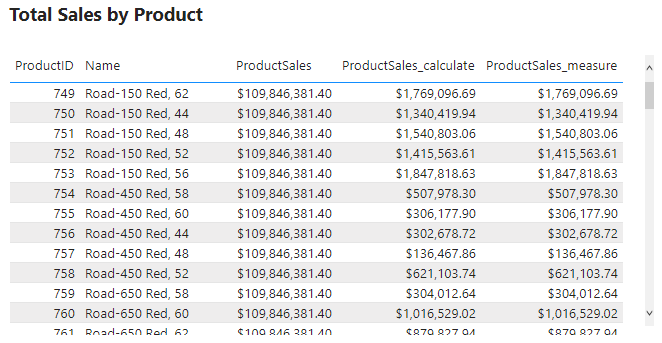
Considering the dataset in our sample report, suppose we want to analyze the overall sales performance, irrespective of any specific regions or dates. Using the following formula, we can provide the total sales amount across all regions and times by removing any existing filters on the Sales table.

All Sales = 
SUMX(
   ALL(Sales), 
   Sales[Amount]
)

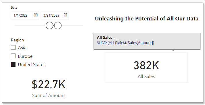
In the above example we can see the card visual on the bottom left is the default sum aggregation of the Amount column in our sales table. Specifically, with the slicers on the report, this card shows the total sales within the United States region during the period between 1/1/2023 and 3/31/2023. We can use the ALL function to display to total sales amount across all regions and irrespective of time, shown on the card visual on the right.

This functionality is particularly useful when making comparative analyses. For instance, we could use this to determine a region’s contribution to total sales. We can compare the sales in a specific region (with filters applied) to the overall sales calculated using ALL. This comparison offers valuable insights into the performance of different segments relative to the total context.


ALLSELECTED Decoded: Interactive Reporting’s Best Friend

The ALLSELECTED function in DAX takes the capabilities of ALL a step further. It is particularly useful in interactive reports where our users apply filters. This function respects the filters applied by our report users but disregards any filter context imposed by report objects like visuals or calculations. The syntax is:

ALLSELECTED([tableName | columnName[, columnName[, columnName[,…]]]] )

Similar to ALL the tableName and columnName parameters are optional and reference an existing table or column, an expression cannot be used. When we provide ALLSELECTED a single argument it can either be tableName or columnName, and when we provide the function more than one argument, they must be columns from the same table.

ALLSELECTED differs from ALL because it retains all filters explicitly set within the query, and it retains all context filters other than row and column filters.

Practical Examples: Exploring ALLSELECTED and How it Differs From ALL

At first glance it may seem as if ALL and ALLSELECTED perform the same task. Although, these two functions are similar there is an important difference between them. ALLSELECTED will ignore filters applied by report visuals, while ALL will ignore any filters applied within the report. Let’s explore this difference with an example.

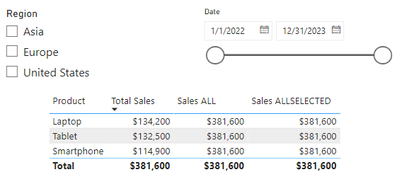
We will use three measures to explore ALLSELECTED. First a measure that simply calculates the sum of our Sales Amount, here is its definition.

Total Sales = SUM(Sales[Amount])

Second a measure using the function explored in the previous section ALL.

Sales ALL = CALCULATE(
    SUM(Sales[Amount]),
    ALL(Sales)
)

Lastly, a measure that uses ALLSELECTED.

Sales ALLSELECTED = 
CALCULATE(
    SUM(Sales[Amount]),
    ALLSELECTED(Sales)
)

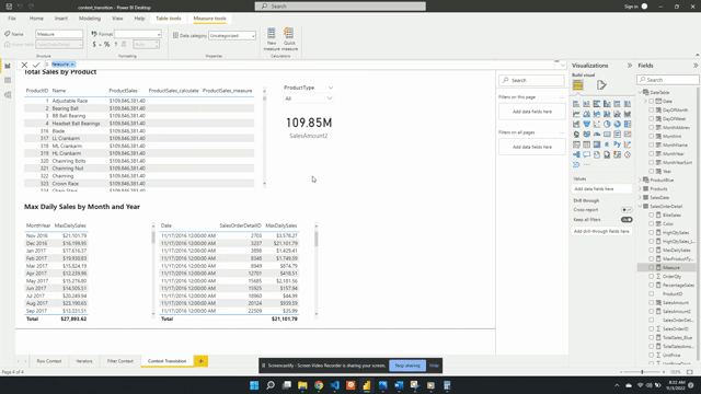
After creating the measures, we can add a table visual including the Product field and these three measures. When the report has no filters due to interacting with the slicers on the report, we can see that the Total Sales measure gets filtered by the Product column and shows the total sales for each product. However, the other two measure show the overall total sales.

The inclusion of the Product column in the table visual is filtering the values and impacting the calculation of the Total Sales measure, while the other two measure are using all of the sales records in their calculation.

Next let’s use the Region and Date slicers to explore the differences between ALL and ALLSELECTED. As expected, all the additional filtering due to the slicer selections continues to impact our Total Sales measure.

Additionally, we see the ALLSELECTED measure gets filtered based on the external slicer selections but continues to not be impacted by the internal filtering of the table visual. This differs from our measure that uses the ALL function, which continues to show the grand total sales value. This is because the ALL function ignores any filter implicit from the visual or explicit from external slicers.

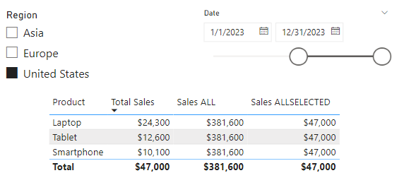
The difference between ALL and ALLSELECTED boils down to ALL will ignore any filter applied, while ALLSELECTED will ignore just the filter applied by the visual.

The necessity of ALLSELECTED is its ability to respect user’s interactions and filtering choices on slicers or other interactive elements. Unlike ALL, which disregards all filters, ALLSELECTED maintains the interactive nature or our reports, ensuring that the calculations dynamically adapt to user inputs.

So, what is a use case for ALLSELECTED? A common use is calculating percentages, based on a total value that is dependent on user interaction with report slicers. Check out this post, on how this function can be used along with ISINSCOPE to calculate context aware insights.

Elevate Your Power BI Report with Context-Aware Insights


CALCULATE: The Engine for Transforming Data Dynamically

CALCULATE is one of the most versatile and powerful functions in DAX, acting as a cornerstone for many complex data operations in Power BI. It allows us to manipulate the filter context of a calculation, letting us perform dynamic and complex calculations with ease. CALCULATE follows a simple structure.

CALCULATE(expression[, filter1[, filter2[, …]]])

The expression parameter is the calculation we want to perform, and the filter parameters are optional boolean expressions or table expression that define our filters or filter modifier functions. Boolean filter expressions are expressions that evaluate to true or false, and when used with CALCULATE there are certain rules that must be followed, see the link below for details. Table filter expressions apply to a table, and we can use the FILTER function to apply more complex filtering conditions, such as those that cannot be defined by using a boolean filter expression. Finally, filter modifier functions provide us even more control when modifying the filter context within the CALCULATE function. Filter modifier functions include functions such as REMOVEFILTERS, KEEPFILTERS, and the ALL function discussed in the previous section.

Find all the required details in the documentation.

Learn more about: CALCULATE

Practical Examples: Using CALCULATE for Dynamic Data Analysis

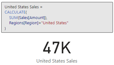
Let’s say that for our report we are required to calculate the total sales in the United States region. We can use CALCULATE and this expression to meet this requirement.

United States Sales = 
CALCULATE(
   SUM(Sales[Amount]), 
   Regions[Region]="United States"
)

We can continue to build on the previous example to further examine sales in the United States. For this example, we will compare the average sales of smartphones in the United States against the benchmark of average sales of smartphones across all regions.

US Smartphone Sales vs. Average Smartphone Sales =
    CALCULATE(
        AVERAGE(Sales[Amount]),
        Products[Product] = "Smartphone",
        Regions[Region] = "United States"
    )
    - AVERAGEX(
        FILTER(
            Sales,
            RELATED(Products[Product]) = "Smartphone"
        ),
        Sales[Amount]
)

These two examples just begin to scratch the surface of what is possible when we utilize the CALCULATE function. For more examples and more details on CALCULATE check out this post that provides a deep dive into the CALCULATE function.

Demystifying CALCULATE: An exploration of advanced data manipulation. 

CALCULATE proves indispensable for redefining the filter context impacting our calculations. It empowers us to perform targeted analysis that goes beyond the standard filter constraints of a report, making it an essential tool in our DAX toolbox.


Mastering FILTER: The Art of Precision in Data Selection

The FILTER function in DAX is a precision tool for refining data selection within Power BI. It allows us to apply specific conditions to a table or column, creating a subset of data that meets the criteria. The FILTER function returns a table that represents a subset of another table or expression, and the syntax is as follows.

FILTER(table, filter)

The table argument is the table, or an expression that results in a table, that we want to apply the filter to. The filter argument is a boolean expression that should be evaluated for each row of the table.

FILTER is used to limit the number of rows in a table allowing for us to create specific and precise calculations. When we use the FILTER function we embed it within other functions, we typically do not use it independently.

When developing our Power BI reports a common requirement is to develop DAX expressions that need to be evaluated within a modified filter context. As we saw in the previous section CALCULATE is a helpful function to modify the filter context, and accepts filter arguments as either boolean expressions, table expression or filter modification functions. Meaning CALCULATE, will accept the table returned by FILTER as one of its filtering parameters, however it is generally best practice to avoid using the FILTER function as a filter argument when a boolean expression can be used. The FILTER function should be used when the filter criteria cannot be achieved with a boolean expression. Here is an article that details this recommended best practice.

Best practices for using the FILTER function as a filter argument.

For example, we have two measures below that calculate the total sales amount for the United States. Both of these measures correctly filter our data and calculate the same value for the total sales. When possible, the best practice is to use the expression on the left which passes the filter arguments to CALCULATE as a boolean expression. This is because when working with Import model tables that are store in-memory column stores, they are explicitly optimized to filter column in this way.

Practical Examples: FILTER Functions Illustrated

Let’s now see how FILTER can help us build on our analysis of US Smartphone Sales. In the previous section we created a US Smartphone Sales vs Average Smartphone Sales measure to visualize US sales against a benchmark. Now we are interested in the total sales amount for each quarter that average US smartphones sales is below the benchmark. FILTER can help us do this with the following expression.

United States Sales FILTER = 
   CALCULATE(
      SUM(Sales[Amount]), 
      FILTER(
         VALUES(DateTable[YearQuarter]), 
         [US Smartphone Sales vs. Average Smartphone Sales] &lt; 0
      )
   )

FILTER is particularly useful when we require a detailed and specific data subset. It is a function that brings granular control to our data analysis, allowing for a deeper and more focused exploration of our data.


Dynamic Table Creation with CALCULATETABLE

The CALCULATETABLE function in DAX is a powerful tool for creating dynamic tables based on specific conditions. This function performs provides us the same functionality that CALCULATE provides, however rather than returning a singular scalar value CALCULATETABLE returns a table. Here is the function’s syntax:

CALCULATETABLE(expression[, filter1[, filter2[, …]]])

This may look familiar, CALCULATETABLE has the same structure as CALCULATE for details on the expression and filter arguments check out the previous section focused on the CALCULATE function.

Practical Examples: Apply CALCULATETABLE

Let’s say we want to calculate the total sales for the current year so we can readily visualize the current year’s sale broken down by product, region and employee. CALCULATETABLE can help us achieve this with the following expression.

Current Year Total Sales = 
SUMX(
   CALCULATETABLE(
      Sales, 
      YEAR(Sales[SalesDate]) = YEAR(TODAY())
   ), 
   Sales[Amount]
)

CALCULATETABLE proves to be invaluable when we need to work with a subset of data based on dynamic conditions. It’s flexibility to reshape our data on the fly makes it an essential function for nuanced and specific data explorations in Power BI.


Resetting the Scene with REMOVEFILTERS

The REMOVEFILTERS function in DAX is crucial for when we need to reset or remove specific filters applied to our data. It allows for recalibration of the filter context, either entirely or partially. The syntax for this function is:

REMOVEFILTERS([table | column[, column[, column[,…]]]])

Looking at the structure of REMOVEFILTERS, we can see it is similar to that of ALL and ALLSELECTED. Although these functions are similar it is important to differentiate them. While ALL removes all filters from a column or table and ALLSELECTED respects user-applied filter but ignores other filter contexts, REMOVEFILTERS specifically targets and removes filters from the specified columns or tables, offering us more control and precision.

Practical Examples: Implementing REMOVEFILTERS

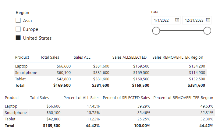
Let’s start by adding a new measure to our previous table visual where we explored the difference between ALL and ALLSELECTED to highlight the difference between these functions.

We will create a new measure and add it to the table visual, the new measure is:

Sales REMOVEFILTER Region = 
CALCULATE(
   SUM(Sales[Amount]), 
   REMOVEFILTERS(Regions[Region])
)

This expression will calculate the total sales disregarding any Region filter that might be in place.

Here we can see this new Sales REMOVEFILTER Region measure shows the total sales respecting the row context of Product on the table visual and the selected dates on the date slicer, however, removes the Region filter that would apply due to the Region slicer.

Let’s take a look at how we can apply and leverage the differences between these functions. We can use our Total Sales and the other three measures to calculate various percentages to provide additional insights.

REMOVEFILTERS offers a tailored approach to filter removal, differing from ALL which disregards all filters unconditionally, and ALLSELECTED which adapts to user selections. This makes REMOVEFILTERS an essential function for creating more nuanced and specific measures in our Power BI reports.


LOOKUPVALUE: Bridging Tables in Analysis

The LOOKUPVALUE function in DAX is a powerful feature for cross-referencing data between tables. It allows us to find a value in a table based on matching a value in another table or column.

LOOKUPVALUE (
    result_columnName,
    search_columnName,
    search_value
    [, search2_columnName, search2_value]…
    [, alternateResult]
)

Here result_columnName is the name of an existing column that contains the value we want to be returned by the function; it cannot be an expression. The search_columnName argument is the name of an existing column and can be in the same table as the result_columnName or in a related table, the search_value is the value to search for within the search_columnName. Finally, the alternativeResult is an optional argument that will be returned when the context for result_columnName has been filter down to zero or more than one district value, when not specified LOOKUPVALUE will return BLANK.

LOOKUPVALUE is essential for scenarios where data relationships are not directly defined through relationships in the data model. If there is a relationship between the table that contains the result column and tables that contain the search column, typically using the RELATED function rather than LOOKUPVALUE is more efficient.

Practical Examples: LOOKUPVALUES Explored

Let’s use LOOKUPVALUE to connect sales data with the respective sales managers. We need to identify the manager for each sale in our Sales table for our report. We can use a formula that first finds the manager’s ID related to each sale. For details on how we can user Parent and Child Functions to work with hierarchical data check out the Parent and Child Functions: Managing Hierarchical Data section of this post.

Unlock the Full Potential of Your Data with DAX: From Basic Aggregations to Advanced Time Intelligence

In the example in the post above we use PATH and PATHITMEREVERSE to navigate the organizational hierarchy to identify the manager’s ID of each employee. Then utilizing REALTED and LOOKUPVALUE we can add a new calculated column to our Sales table listing the Sales Manager for each sale. We can use the following formula that first finds the manager’s ID related to each sale and then fetches the manager’s name using the LOOKUPVALUE function.

Sales Manager Name = 
VAR ManagerID = RELATED(Employee[ManagerID])

RETURN
LOOKUPVALUE(Employee[EmployeeName], Employee[EmployeeID], ManagerID)

In this example, the RELATED function retrieves the ManagerID for each sale from the Employees table. Then, LOOKUPVALUE is used to find the corresponding EmployeeName (the manager’s name) in the same table based on the ManagerID. This approach is particulariy beneficial in scenarios where understanding hierarchical relationships or indirect associations between data points is crucial.

By using LOOKUPVALUE in this manner, we add significant value to our reports, offering insights into the managerial oversight of sales activities, which can be pivotal for performance analysis and strategic planning.


Mastering DAX Filter Functions for Advanced Analysis

Now that we have finished our exploration of DAX Filter Functions in Power BI, it is clear that these tools are not just functions, they are the building blocks for sophisticated data analysis. From the comprehensive clearing of contexts with ALL to dynamic and context-sensitive capabilities of CALCULATE and FILTER, each function offers a unique approach to data manipulation and analysis.

Understanding and applying functions like ALLSELECTED, REMOVEFILTERS and LOOKUPVALUE enable us to create reports that are not only insightful but also interactive and responsive to user inputs. They allow use to navigate through complex data relationships with ease, bringing clarity and depth to our analyses.

As we continue our journey in data analytics, remember that mastering these functions can significantly enhance our ability to derive meaningful insights from our data. Each function has its place and purpose, and knowing when and how to use them will set us apart as proficient Power BI analyst.

Embrace these functions as we delve deeper into our data and watch as they transform our approach to business intelligence and data storytelling. Happy analyzing!


Thank you for reading! Stay curious, and until next time, happy learning.

And, remember, as Albert Einstein once said, “Anyone who has never made a mistake has never tried anything new.” So, don’t be afraid of making mistakes, practice makes perfect. Continuously experiment and explore new DAX functions, and challenge yourself with real-world data scenarios.

If this sparked your curiosity, keep that spark alive and check back frequently. Better yet, be sure not to miss a post by subscribing! With each new post comes an opportunity to learn something new.

ISINSCOPE: The Key to Dynamic Data Drilldowns


Welcome, to another journey through the world of DAX, in this post we will be shining the spotlight on the ISINSCOPE function. If you have been exploring DAX and Power BI you may have encountered this function and wondered its purpose. Well, wonder no more! We are here to unravel the mysteries and dive into some practical example showing just how invaluable this function can be in our data analysis endeavors.

If you are unfamiliar DAX is the key that helps us unlock meaningful insights. It is the tool that lets us create custom calculations and serve up exactly what we need. Now, lets focus on ISINSCOPE, it is a function that might not always steal the show but plays a pivotal role, particularly when we are dealing with hierarchies and intricate drilldowns in our reports. It provides us the access to understand at which level of hierarchy our data is hanging out, ensuring our calculations are always in tune with the context.

For those of you eager to start experimenting there is a Power BI report pre-loaded with the sample data used in this post ready for you. So don’t just read, follow along and get hands-on with DAX in Power BI. Get a copy of the sample data file (power-bi-sample-data.pbix) here:

This dynamic repository is the perfect place to enhance your learning journey.


Exploring the ISINSCOPE Function

Let’s dive in and get hand on with the ISINSCOPE function. Think of this function as our data GPS, it helps us figure out where we are in the grand scheme of our data hierarchies.

So, what exactly is ISINSCOPE? In plain terms, it is a DAX function used to determine if a column is currently being used in a specific level of a hierarchy or, put another way, if we are grouping by the column we specify. The function returns true when the specified column is the level being used in a hierarchy of levels. The syntax is straightforward:

ISINSCOPE(column_name)

The column_name argument is the name of an existing column. Just add a column that we are curious about, and ISINSCOPE will return true or false depending on whether that column is in the current scope.

Let’s use a simple matrix containing our Region, Product Category, and Product Code to set up a hierarchy and see ISINSCOPE in action with the following formula.

ISINSCOPE = 
SWITCH(
    TRUE(),
    ISINSCOPE(Products[Product Code]), "Product Code",
    ISINSCOPE(Products[Product]), "Product",
    ISINSCOPE(Regions[Region]), "Region"
)

This formula uses ISINSCOPE in combination with SWITCH to determine the current context, and if true returns a text label indicating what level is in context.

But why is this important? Well, when we are dealing with data, especially in a report or a dashboard, we want our calculations to be context-aware. We want them to adapt based on the level of data we are looking at. ISINSCOPE allows us to create measures and calculated columns that behave differently at different levels of granularity. This helps provide accurate and meaningful insights.


Diving Deeper: How ISINSCOPE Works

Now that we have got a handle on what ISINSCOPE is, let’s dive a bit deeper and see how it works. At the heart of it ISINSCOPE is all about context, specifically, row context and filter context.

For an in depth look into Row Context and Filter Context check out the posts below that provide all the details.

Row Context — What it is, When is it available, and its Implications

Filter Context – How to create it and its impact on measures

For our report we are interested in analyzing the last sales date of our products, and want this information in a matrix similar to the example above. We can easily create a Last Sales Date measure using the following formula and add it to our matrix visual.

Last Sales Date = MAX(Sales[SalesDate])

This provides a good start, but not quite what we are looking for. For our analysis the last sales date at the Region level is too broad and not of interest, while the sales date of Product Code is too granular and clutters the visual. So, how do we display the last sales date just at the Product Category (e.g. Laptop) level? Enter ISINSCOPE.

Let’s update our Last Sales Date measure so that it will only display the date on the product category level. Here is the formula.

Product Last Sales Date = 
SWITCH(
    TRUE(), 
    ISINSCOPE(Products[Product Code]), BLANK(), 
    ISINSCOPE(Products[Product]), FORMAT(MAX(Sales[SalesDate]),"MM/dd/yyyy"), 
    ISINSCOPE(Regions[Region]), BLANK()
)

We use SWITCH in tandem with ISINSCOPE to determine the context, and if Product is in context the measure returns the last sales date for that product category. However, at the Region and Product Code levels the measure will return a blank value.

The use of ISINSCOPE helps enhance the matrix visual preventing it from getting over crowded with information and ensuring that the information displayed is relevant. It acts as a smart filter, showing or hiding data based on where we are in a hierarchy, making our reports more intuitive and user-friendly.


ISINSCOPE’s Role in Hierarchies and Drilldowns

When we are working with data, understanding the relationship between parts and the whole is crucial. This is where hierarchies and drilldowns come into play, and ISINSCOPE is the function that helps us make sense of it all.

Hierarchies allow us to organize our data in a way that reflects real-world relationships, like breaking down sales by region, then product category, then specific products. Drilldowns let us start with a broad view and then zoom in on the details. But how do we keep our calculations accurate at each level? You guessed it, ISINSCOPE.

Let’s look at a DAX measure that leverages ISINSCOPE to calculate the percentage of sales each child represents of the parent in our hierarchy.

Percentage of Parent = 
    VAR AllSales = 
        CALCULATE(Sales[Total Sales], ALLSELECTED())
    VAR RegionSales = 
        CALCULATE([Total Sales], ALLSELECTED(), VALUES(Regions[Region]))
    VAR RegionCategorySales = 
        CALCULATE([Total Sales], ALLSELECTED(), VALUES(Regions[Region]), VALUES(Products[Product]))
    VAR CurrentSales = [Total Sales]

RETURN
SWITCH(TRUE(),
    ISINSCOPE(Products[Product Code]), DIVIDE(CurrentSales, RegionCategorySales),
    ISINSCOPE(Products[Product]), DIVIDE(CurrentSales, RegionSales),
    ISINSCOPE(Regions[Region]), DIVIDE(CurrentSales, AllSales)
)

The Percentage of Parent measure uses ISINSCOPE to determine the current level of detail we are working with. If we are viewing our sales by region the measure calculates the sales for the region as a percentage of all sales.

But the true power of ISINSCOPE begins to reveal itself as we drilldown into our sales data. If we drilldown into each region to show the product categories we see that the measure will calculate the sales for each product category as a percentage of sales for that region.

And then again, if we drilldown into each product category we can see the measure will calculate the the sales of each product code as a percentage of sales for that product category within the region.

By incorporating this measure into our report, we help ensure that as we drilldown into our data the percentages are always calculated relative to the appropriate parent in our hierarchy. This allows us to provide accurate measures that provide the appropriate context, making our reports more intuitive and insightful.

ISINSCOPE is the key element to maintaining the integrity of our hierarchical calculations. It ensures that as we navigate through different levels of our data our calculations remain relevant and precise, providing a clear understanding of how each part contributes to the whole.


Best Practices for Leveraging ISINSCOPE

When it comes to DAX and ISINSCOPE a few best practices can ensure that our reports are accurate, performant, and user-friendly. Here are just a few things that can help us make the most out of ISINSCOPE:

  1. Understand Context: Before using ISINSCOPE, make sure to have a solid understanding of row and filter context. Knowing which context we are working with will help us use ISINSCOPE effectively.
  2. Keep it Simple: Start with simple measures to understand how ISINSCOPE behaves with our data. Complex measures can be built up gradually as we become more comfortable with the function.
  3. Use Variables: Variables can make our DAX formulas easier to read and debug. They also help with performance because they store a result of a calculation for reuse.
  4. Test at Every Level: When creating measures with ISINSCOPE, test them at every level, this helps ensure that our measures work correctly no matter how the users interact with the report.
  5. Combine with Other Functions: ISINSCOPE is often used in combination with other DAX functions. Learning how it interacts with functions like SWITCH, CALCULATE, FILTER, and ALLSELECTED will provide us more control over our data.

Wrapping up

Throughout our exploration of the ISINSCOPE function we have uncovered its pivotal role in managing data hierarchies and drilldowns providing for accurate and context-sensitive reporting. Its ability to discern the level of detail we are working with allows for dynamic measures and visuals that adapt to user interactions, making our reports not just informative but interactive and intuitive.

With practice, ISINSCOPE will become a natural part of your DAX toolkit, enabling you to create sophisticated reports that meet the complex needs of any data analysis challenge you might face.

For those looking to continue their journey into DAX and its capabilities there is a wealth of resources available, and a good place to start is the DAX Reference documentation.

Learn more about: Power Automate Excel Online (Business) Actions

I have also written about other DAX functions including Date and Time Functions, Text Functions, an entire post focused on the CALCULATE function and an ultimate guide providing a overview of all the DAX function groups.

Explore the ebb and flow of the temporal dimension of your data with DAX’s suite of Date and Time Functions.

Stringing Along with DAX: Dive Deep into Text Expressions

Demystifying CALCULATE: An exploration of advanced data manipulation. 

Unlock the Full Potential of Your Data with DAX: From Basic Aggregations to Advanced Time Intelligence


Thank you for reading! Stay curious, and until next time, happy learning.

And, remember, as Albert Einstein once said, “Anyone who has never made a mistake has never tried anything new.” So, don’t be afraid of making mistakes, practice makes perfect. Continuously experiment and explore new DAX functions, and challenge yourself with real-world data scenarios.

If this sparked your curiosity, keep that spark alive and check back frequently. Better yet, be sure not to miss a post by subscribing! With each new post comes an opportunity to learn something new.

Power BI Context Transition: Navigating the Transition between Row and Filter Contexts

Series Review

One of the early stages of creating any Power BI report is the development of the data model. The data model will consist of data tables, relationships, and calculations. There are two types of calculations: calculated columns, and measures.

Check out Power BI Row Context: Understanding the Power of Context in Calculations for key differences between calculated columns and measures.

Row Context — What it is, When is it available, and its Implications

One of the most powerful elements of Power BI is that all measure calculations are done in context. The evaluation context limits the values in the current scope when evaluating an expression. The filter context and/or the row context make up the evaluation context.

Power BI Row Context: Understanding the Power of Context in Calculations of this series explores the row context in depth.

While Power BI Iterators: Unleashing the Power of Iteration in Power BI Calculations explores iterator functions, which are functions that create row context.

Iterator Functions — What they are and What they do

And finally, Power BI Filter Context: Unraveling the Impact of Filters on Calculations explores the concept of the filter context.

Filter Context – How to create it and its impact on measures

When evaluating expressions, the row context can be transitioned into a filter context within Power BI. This transition can help create more complex measures. Row context, filter context, and context transition can be confusing when starting with DAX so visit references and documentation often.

This post is the fourth of a Power BI Fundamental series with a focus on the context transition. The example file used in this post is can be found on GitHub at the link below.

Power BI key fundamentals example files


Understanding Context Transition

The row context by itself does not filter data. Row context iterates through a table row-by-row. Context transition is when the row context transitions into the filter context. Context transition occurs with the CALCULATE() function and when the expression of an iterator function is a DAX measure.

The concept of context transition can be a bit abstract so it can be easiest to learn through examples. To explore, we will create a new calculated column in the Products table. The new ProductsSales calculates the total sales for each product and we define it as:

ProductSales = 
SUM(SalesOrderDetail[SalesAmount])

After evaluating ProductSales we see it repeats the same $109.85M sales value for each row. This value is the total sales amount for the entire dataset. This is not what we want ProductSales to calculate, so what happened?

ProductSales calculates the total sales of the entire data rather than the filtered per-product value because row context is not a filter. For example, the row context includes the ProductID value but this identifier is not a filter on the data during evaluation. And because the row context is not a filter DAX does not distinguish between different rows (i.e products) when evaluating ProductSales.

For example, looking at the table above while evaluating the measure DAX does not distinguish the Adjustable Race row from the LL Crankarm row. Since all rows are viewed as the same the total sales value is repeated for each row.

You may have guessed it but, the example above calculates the wrong value because it does not contain a context transition. The row context does not shift to the filter context causing the error in the calculated value. This simple example highlights why context transition is important and when it’s needed. To correct this we must force the context transition. This will convert the row values into a filter and calculate the sales for each product. There are various ways to do this, and below are two options.

Option #1: The CALCULATE() Function

We can force context transition by wrapping ProductSales with the CALCULATE() function. To demonstrate we create a new ProductSales_calculate column. ProductSales_calculate is defined as:

ProductSales_calculate = 
CALCULATE(
   SUM(SalesOrderDetail[SalesAmount])
)

This new calculated column shows the correct sales value for each product. We view the product type BK and can see now each row in the ProductSales_calculate column is different for each row.

Option #2: Using Measures

Within the data model, we have already created a measure SalesAmount2.

We defined SalesAmount2 as:

SalesAmount2 = 
SUMX(
   SalesOrderDetail, 
   SalesOrderDetail[OrderQty] * SalesOrderDetail[UnitPrice] * (1 - 
   SalesOrderDetail[UnitPriceDiscount])
)

We can see by the expression SalesAmount2 uses the iterator function SUMX(). This measure calculates the sales amount row-by-row in the SalesOrderDetail table. As mentioned before context transition occurs within iterator functions. So rather than using CALCULATE() and SUM() we create another calculated column that references this measure.

ProductSales_measure = SalesAmount2

We add the new column to the table visual and can see that it has the same value as ProductSales_calculate. This shows that a measure defined with an iterator also forces context transition.

An important note about this new column is that the ProductsSales_measure works as expected when referencing the measure. However, it will not work if we define this column as the same expression that defines SalesAmount2.

We can see below if we update ProductSales_measure to:

SUMX(
   SalesOrderDetail, 
  SalesOrderDetail[OrderQty] * SalesOrderDetail[UnitPrice] * (1 - 
  SalesOrderDetail[UnitPriceDiscount])
)

The same expression used when defining SalesAmount2, will result in wrong values.

After updating ProductSales_measure we can see it returns the total sales values and not the sales per product. With this updated definition DAX is no longer able to apply the context transition. We can correct this by wrapping the expression with CALCULATE().


Maximum Daily Sales by Month Example

A question of interest is what is the maximum daily sales amount for each month in the dataset. In other words we would like to determine for each month what day of the month had the highest sales and what was the total daily sales value. We start by creating a new MaxDailySales measure and add it to the Max Daily Sales by Month and Year table visual.

We define MaxDailySales as:

MaxDailySales = 
MAXX(SalesOrderDetail, [SalesAmount2])

After adding the measure to the table we can see the sales amount value for each month. For example, the table currently shows that the maximum daily sales for November 2016 is $21,202.79. This value may appear reasonable but when examined closely we can determine it is incorrect. Currently, MaxDailySales is returning the maximum sale for each month and is not accounting for multiple sales within each day. We can see this by creating a new visual with the Date, MaxSales, and SalesOrderDetailID fields.

This table shows that the MaxDailySales for November 2016 is the same value as a single sale that occurred on November 17th. Yet, there are multiple sales on this day and every other day. The desired outcome is to calculate the total sales for each day and then determined the highest daily total value for each month.

This error occurs because context transition is not being applied correctly. It is important to note that context transition is occurring while evaluating MaxDailySales because it is a measure. However, the context transition is not being applied on the correct aggregation level. The context transition is occurring on the SalesOrderDetail level, meaning for each row of this table. To correct this measure we will have to force the context transition on the correct, daily, aggregation level. We update the MaxDailySales expression using the VALUES() function.

We define MaxDailySales_Corrected as:

MaxDailySales_Corrected = 
MAXX(
   VALUES(DateTable[Date]), 
   [SalesAmount2]
)

We change the table passed to MAXX() from SalesOrderDetail to VALUES(DateTable[Date]). Using VALUES(DateTable[Date]) aggregates all the dates that are the same day shifting the context transition to the correct aggregation level. The VALUES() function in the expression provides a unique list of dates. For each day in the unique list, the SalesAmount2 measure gets evaluated and returns the maximum daily total value. We then add the new measure to the table visual and now it shows the correct maximum daily sales for each month.

The above example shows context transition at two different aggregation levels. They also highlight that the context transition can be shifted to return the specific value that is required. As well as showing why it is important to take into consideration the aggregation level when developing measures like MaxDailySales.


Context Transition Pit Falls

Context transition is when row values transition into or replace the filter context. When context transition occurs it can sometimes lead to unexpected and incorrect values. An important part of context transition to understand is that it transitions the entire row into the filter. So what occurs when a row is not unique? Let’s explore this with the following example.

We add a new SimplifiedSales table to the data model.

Then we add a TotalSales measure. TotalSales is defined as:

TotalSales = 
SUMX(
   SimplifiedSales, 
   SimplifiedSales[OrderQty] * SimplifiedSales[UnitPrice] * (1 - 
   SimplifiedSales[UnitPriceDiscount])
)

Viewing the two tables above, we can confirm that the TotalSales values are correctly aggregating the sales data. Now we add another measure to the table which references the measure TotalSales. Referencing this measure will force context transition due to the implicit CALCULATE() added to measures. See above for details.

We define TotalSales_ConextT as:

TotalSales_ContextT = 
SUMX(SimplifiedSales, [TotalSales])

In the new column we can see that the values for Road-350-W Yellow, 48 and Touring-3000 Blue, 44 have not changed and are correct. However, Mountain-500 Silver, 52 did update, and TotalSales_ContextT column shows an incorrect value. So what happened?

The issue is the context transition. Viewing the SimplifiedSales table we can see that Mountain-500 Silver, 52 appears twice in the table. With both records having identical values for each field. Remember, context transition utilizes the entire row. Meaning the table gets filtered on Mountain-500 Silver, 52/ 1/$450.00. Because of this, the result gets summed up in the TotalSales measure returning a value of $900.00. This value is then evaluated twice, once for each identical row.

This behavior is not seen for the Road-350-W, 48 records because they are unique. One row has a UnitPriceDiscount of 0.0% and the other has a value of 5.0%. This difference makes each row unique when context transition is applied.

Knowing what context transition is and when it occurs is important to identifying when this issue may occur. When context transition is applied it is important to check the table and verify calculations to ensure it is applied correctly.


Thank you for reading! Stay curious, and until next time, happy learning.

And, remember, as Albert Einstein once said, “Anyone who has never made a mistake has never tried anything new.” So, don’t be afraid of making mistakes, practice makes perfect. Continuously experiment and explore new DAX functions, and challenge yourself with real-world data scenarios.

If this sparked your curiosity, keep that spark alive and check back frequently. Better yet, be sure not to miss a post by subscribing! With each new post comes an opportunity to learn something new.

Power BI Iterators: Unleashing the Power of Iteration in Power BI Calculations

Overview

In order to facilitate analysis and visualization in Power BI a data model must first be created. The data model consists of individual data tables, relationships, and calculations. Calculations come in the form of either calculated columns or measures.

Check out this post to explore the key differences between calculated columns and measures.

Row Context — What it is, When is it available, and its Implications

The evaluation context limits the values in the current scope when Power BI evaluates a DAX expression. There are two types of evaluation context, filter and row, that can be active during the evaluation of a DAX expression.

This post is the second of a Power BI Fundamental series with a focus on iterator functions. The example file used in this post is located found on GitHub at the link below.

Power BI key fundamentals example files


Introduction

This post will build upon the Power BI file created in Part 1 of the series titled row_context_example. The example file for this post is iterator_functions, and both can be found on GitHub at the link above.

As noted at the end of Power BI Row Context: Understanding the Power of Context in Calculations, creating a measure by default was unable to reference the row values of a column. When creating a measure a column can be referenced and passed to a standard aggregation function. The standard aggregation function will return only a single aggregated value. This is not the row-by-row functionality that will be required to replace a calculated column, such as SalesAmount found in the SalesOrderDetail table.

Creating the desired measure will require an iterator function to create row context.

Understanding Iterators

An iterator moves row-by-row or iterates through an object. The object can be a data model table or a virtual/temporary table. Data model tables are tables loaded into or linked to within Power BI. A table generated from within a measure that persists only for a temporary period of time is a virtual table.

An iterator function can return a single value (e.g. number, text, date) or a virtual table. An iterator generally has two arguments:

  • The object (i.e. table) to iterate through
  • The expression evaluated for each row of the object

It can be helpful to think of the expression as a temporary column of the object. Evaluation of the expression occurs row-by-row creating a column of calculated results. The column of results only persists during the evaluation and is not loaded to the data model. The purpose of the temporary column is to calculate the final returned value of the iterator.

Examples of iterator functions include SUMXMINXMAXXAVERAGEX, and RANKX. The ending X is only a common identifier, FILTER is an example of an iterator function that does not end with a X.

Example iterator function:

SUMX(
   SalesOrderDetail, 
   SalesOrderDetail[OrderQty] * SalesOrderDetail[UnitPrice] * (1 - SalesOrderDetail[UnitPriceDiscount])
)
  • Table: SalesOrderDetail – the object iterated over
  • Expression: SalesOrderDetail[OrderQty] * SalesOrderDetail[UnitPrice] * (1 - SalesOrderDetail[UnitPriceDiscount]) – the expression evaluated for each row.

Once implementing the iterator SUMX and specifying the table as SalesOrderDetails the columns of the table will be recognized and able to be referenced like when a calculated column was created. The new measure SalesAmount2 created using an iterator will replace the calculated column SalesAmount. Comparing the default aggregation of the SalesAmount column (i.e. Sum of SalesAmount) and the new measure SalesAmount2 it can been see the values are equal.


Iterator Functions that Generate Virtual Tables

There are iterator functions such as SUMX that return a scalar value and there are ones like FILTER that return virtual tables.

To further explore, first create a new table in the data model generated by the returned table of the FILTER function.

For this example, we use the FILTER function to create a new ProductBlue table. For the first argument of the FILTER function we pass in the Product table. Then we filter that table using a filter expression defined as Products[Color] = "blue".

ProductBlue = FILTER(Products, Products[Color] = "blue")

We then can visualize this new table and compare the row count to the count of ProductID by color of the original table. Comparing these two tables we see that ProductBlue is a subset of the Product table.

The generation of this table highlights the iterating functionality and the row context when evaluating the FILTER function. To create the ProductBlue table the FILTER iterator function must create row context. During the evaluation, the function must go within the Products table and for each row (i.e. row context) evaluate what the product color is. If the color is Blue the function returns True otherwise returns False. The resulting table then consists of only rows from the original table which evaluated to a value of True.

Creating the new ProductBlue table was for demonstrative purposes. The table returned by FILTER can be a virtual table used within a measure. In this case, the ProductBlue table would only persist while the measure is being evaluated. As an example, create a new ProductBlueMeasure measure using the COUNTROWS function. COUNTROWS takes a single argument, the table to count the row of. To do this we will pass the FILTER expression used to create the ProductBlue table to the COUNTROWS function. To further demonstrate that the ProductBlue table is unnecessary, we can create a similar ProductBlackMeasure by changing =”blue" to =”black". Viewing these measures shows the result is the same counts that were produced by the other methods used to obtain this count.


Combining Iterators

More complex measures can be created by combining or nesting iterators. For example, combining the product color and the sales data, such as evaluating the total sales for only blue products. This measure will first create a virtual table of the sales data for only blue products. Then iterate row-by-row through the virtual table and evaluate the sales amount. Finally, return the total sales amount.

The DAX expression will be:

SUMX(
   FILTER(
      SalesOrderDetail, 
      RELATED(Products[Color])="Blue"
   ), 
  SalesOrderDetail[OrderQty] * SalesOrderDetail[UnitPrice] * (1 - SalesOrderDetail[UnitPriceDiscount])
)

The virtual table mentioned above is generated by FILTER(SalesOrderDetail, RELATED(Products[Color])="Blue").
This is the first iterator function that is evaluated using the SalesOrderDetail table and the expression RELATED(Products[Color])="Blue".

RELATED() is a function that returns a related value from another table. This function can be used since the Product table is related to the SalesOrderDetail table with a key value of ProductID. The FILTER function then returns a subset of the SalesOrderDetail table containing only rows where the product is blue. This virtual table is then passed to SUMX.

Then the expression evaluated row-by-row is:

SalesOrderDetail[OrderQty] * SalesOrderDetail[UnitPrice] * (1 - SalesOrderDetail[UnitPriceDiscount])

Which returns the total sales amount for each row. Then this temporary column is summed by the SUMX function.

Viewing the two tables on the left, the totals sales for the Blue products for all methods is approximately 9.60M. Selecting the blue row in the top table filters the table below, to show sales by Product for only blue products. Viewing the totals for all three methods also shows a value of approximately 9.60M. Lastly, viewing the value card under Nested Iterator shows that the above created DAX expressions results in the same value of 9.60M.

Key concepts are highlighted in the above example

  • Both SUMX and FILTER create row context
  • The FILTER function returns a virtual table which is a subset of SalesOrderDetail
  • SUMX returns the sum of the row-by-row calculation of the sale amount
  • The table passed to SUMX is the table that is returned by the FILTER function, this table only persists during the evaluation of SUMX

The concept of evaluation context has been mentioned in this post as well as in the previous post – Power BI Row Context: Understanding the Power of Context in Calculations.

Row Context — What it is, When is it available, and its Implications

Evaluation context is the context in which a DAX formula evaluates a calculation. There are two types, Power BI Row Context: Understanding the Power of Context in Calculations explored the first type, row context. This post explored iterators or specific functions which create row context to perform multi-column calculations. Check out Part Three of this series which will explore the second type of evaluation context, the filter context.

Filter Context – How to create it and its impact on measures


Thank you for reading! Stay curious, and until next time, happy learning.

And, remember, as Albert Einstein once said, “Anyone who has never made a mistake has never tried anything new.” So, don’t be afraid of making mistakes, practice makes perfect. Continuously experiment and explore new DAX functions, and challenge yourself with real-world data scenarios.

If this sparked your curiosity, keep that spark alive and check back frequently. Better yet, be sure not to miss a post by subscribing! With each new post comes an opportunity to learn something new.