Dive into DAX: Unlock the Full Potential of FORMAT


I recently participated in a data challenge and used it to explore dynamic titles and subtitles in the final report. Dynamic titles provide context, guide users to key insights, and create a more interactive experience.

Dynamic titles were created by developing DAX measures that utilized various DAX functions, including FORMAT. The DAX FORMAT function proved to be a valuable tool in crafting these dynamic elements. FORMAT enables us to produce polished and audience-friendly text, all while leveraging the power of DAX measures.

This guide dives deep into the capabilities of the FORMAT function. We will explore how to use predefined numeric and date formats for quick wins, uncover the secrets of custom numeric and date/time formats, and highlight practical examples that bring clarity to our Power BI visualizations.


The Basics of FORMAT

The FORMAT function in DAX is a valuable tool for customizing the display of data. Its syntax is straightforward:

FORMAT(<value>, <format_string>[, <locale_name>])

In this syntax, <value> represents a value or expression that evaluates to a single value we want to format. The <format_string> is a string that defines the formatting template and <locale_name> is an optional parameter that specifies the locale for the function.

The FORMAT function enables us to format dates, numbers, or durations into standardized, localized, or customized textual formats. This function allows us to define how the <value> is visually represented without changing the underlying data.

It’s important to note that when we use FORMAT, the resulting value is converted to a string (i.e. text data type). As a result, we cannot use the formatted value in visuals that require a numeric data type or in additional numerical calculations.

Power BI offers a Dynamic Format Strings for measures preview feature that allows us to specify a conditional format string that maintains the numeric data type of the measure.

Learn more about: Dynamic Format strings for measures

Since FORMAT converts the value to a string, it easily combines with other textual elements, making it ideal for creating dynamic titles.


Numeric Formats

The predefined numeric formats allow for quick and consistent formatting of numerical data.

General Number: Displays the value without thousand separators.

Currency: Displays the value with thousand separators and two decimal places. The output is based on system locale settings unless we provide the <locale_name> parameter.

Fixed: Displays the value with at least one digit to the left and two digits to the right of the decimal place.

Standard: Displays the value with thousand separators, at least one digit to the left and two to the right of the decimal place.

Percent: Displays the value multiplied by 100 with two digits to the right of the decimal place and a percent sign appended to the end.

Scientific: Displays the value using standard scientific notation.

Yes/No: Displays the value as No if the value is 0; otherwise, displays Yes.

True/False: Displays the value as False if the value is 0; otherwise, displays True.

On/Off: Displays the value as Off if the value is 0; otherwise, displays On.

Predefined formats are ideal for quick, standardized formatting without requiring custom format strings.

Custom Numeric Formats

Predefined numeric formats work well for standard situations, but sometimes, we need more control over how data is displayed. Custom numeric formats enable us to specify exactly how a numeric value appears, providing the flexibility to meet unique scenarios and requirements.

Custom numeric formats use special characters and patterns to define how numbers are displayed. The custom format expression may consist of one to three format strings, separated by semicolons.

When a custom format expression contains only one section, that format is applied to all values. However, if a second section is added, the first section formats positive values, while the second formats negative values. Finally, if a third section is included, it determines how to format zero values.

Here is a summary of various characters that can be used to define custom numeric formats.

0 Digit placeholder: Displays a digit or a zero, pads with zeros as needed, and rounds where required.

# Digit placeholder: Displays a digit or nothing and skips leading and trailing zeros if needed.

. Decimal placeholder: Determines how many digits are displayed to the left and right of the decimal separator.

, Thousand separators: adds a separator or scales the numbers based on usage. Consecutive , not followed by 0 before the decimal place divides the number by 1,000 for each comma.

% Percentage placeholder: Multiplies the number by 100 and appends %

- + $ Display literal character: Display the literal character, to display characters other than -, +, or $ proceed it with a backslash (\) or enclose it in double quotes (" ").
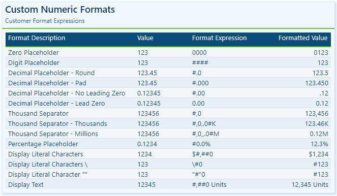
Visit the FORMAT function documentation for additional details on custom numeric formats.

Learn more about: custom numeric format characters that can be specified in the format string argument

Custom numeric formats allow us to present numerical data according to specific reporting requirements. When utilizing custom numeric formats, it is typically best to use 0 for mandatory digits and # for optional digits, include , and . to improve readability, and combine with symbols such as $ or % for intuitive displays.


Date & Time Formats

Dates and times are often key elements in our Power BI reports as they form the basis for timelines, trends, and performance comparisons. The FORMAT function provides several predefined date and time formats to simplify the presentation of date and time values.

General Date: Displays a date and/or time, with the date display determined by the application’s current culture value.

Long Date: Displays the date according to the current culture’s long date format.

Medium Date: Displays the date according to the current culture’s medium date format.

Short Date: Displays the date according to the current culture’s short date format.

Long Time: Displays the time according to the current culture’s long-time format, typically including hours, minutes, and seconds.

Medium Time: Displays the time in a 12-hour format.

Short Time: Displays the time in a 24-hour format.

Predefined formats offer a quick and simple way to standardize date and time outputs that align with current cultural settings.

Custom Date & Time Formats

When the predefined date and time formats don’t meet our requirements, we can utilize custom formats to have complete control over how dates and times are displayed. The FORMAT function supports a wide range of custom date and time format strings.

d, dd, ddd, dddd Day in numeric or text format: single digit (d), with leading zero (dd), abbreviated name (ddd), or full name (dddd).

w Day of the week as a number (1 for Sunday through 7 for Saturday).

ww Week of the year as a number.

m, mm, mmm, mmmm Month in numeric or text format: single digit (m), with leading zero (mm), abbreviated name (mmm), or full name (mmmm).

q Quarter of the year as a number (1-4)

y Display the day of the year as a number.

yy, yyyy Display the year as a 2-digit (yy) number of a 4 digit (yyyy) number.

c Displays the complete date (ddddd) and time (ttttt).

Visit the FORMAT function documentation for additional details and format characters.

Learn more about: custom date/time format characters that can be specified in the format string


Practical Examples in Power BI

Dynamic elements elevate our Power BI visuals by making them context-aware and responsive to user selections. They guide users through the report and help shape the data narrative. The FORMAT function in DAX is one tool we can use to craft these dynamic elements, which allows us to combine formatted values with descriptive text.

Here are three examples where the FORMAT function can have a significant impact.
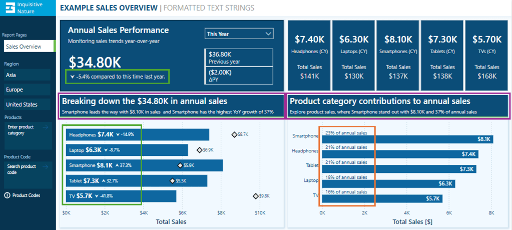
Enhancing Data Labels

At times, numbers alone do not effectively convey insights. Enhancing our labels with additional text features, such as arrows or symbols to indicate trends like growth or decline, can greatly improve their informative value.

In this report, we have a card visual that presents both the annual performance and year-over-year (YoY) performance.

Let’s look at how the FORMAT function was used to achieve this.

The YoY Measure

The Power BI data model includes a measure called Sales Metric YOY, which calculates the percentage change between the selected year and the previous year.

Sales Metric YOY = 
VAR _cy = [Sales Metric (CY)]
VAR _ly = [Sales Metric (LY)]

RETURN
IF(
    ISBLANK(_cy) || ISBLANK(_ly),
    BLANK(),
    DIVIDE(_cy-_ly, _ly)
)

The measure is formatted as a percentage and displays as expected when added to our visuals.
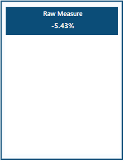
We then use this measure to create an enhanced label. If the value is positive, we add an upward arrow to indicate growth, and if the value is negative, we include a downward arrow to signify decline.

Adding the arrow text elements to the label can be done with the following expression.

Sales Metric YOY Label No Format = 
If(
 [Sales Metric YOY]>0, 
    UNICHAR(11165) & " " & [Sales Metric YOY],
    UNICHAR(11167) & " " & [Sales Metric YOY]
)

However, when we combine our Sales Metric YOY measure with textual elements, we lost the percentage formatting, making the value less user-friendly.

To address this, we can manually multiply the value by 100, round it to one decimal place, and add a % at the end.

Sales Metric YOY Label Manual = 
If(
 [Sales Metric YOY]>0, 
    UNICHAR(11165) & " " & ROUND([Sales Metric YOY]*100, 1)& "%",
    UNICHAR(11167) & " " & ROUND([Sales Metric YOY]*100 ,1) & "%"
)

This expression can be greatly improved by leveraging the power of the FORMAT function. The following expression uses FORMAT to create the enhanced label in a simpler manner for better clarity.

Sales Metric YOY Label = 
If(
 [Sales Metric YOY]>0, 
    UNICHAR(11165) & " " & FORMAT([Sales Metric YOY], "#0.0%"),
    UNICHAR(11167) & " " & FORMAT([Sales Metric YOY], "#0.0%")
)

We can then use the Sales Metric YoY Label throughout our report, such as a data label detail in our bar chart displaying the annual sales by product category and each product’s YoY Label.

To finalize the label in our Annual Sales Performance card, we combine the Saless Metric YoY Label with additional context based on the user’s selected year.

Annual Sales Performance Label = 
[Sales Metric YOY Label] & 
If(SELECTEDVALUE(DateTable[Year Category]) = "This year",
    " compared to this time last year.",
    " compared to " & YEAR(MAX(DateTable[Date])) - 1 & " sales."
)

We now have a dynamic and informative label that we can use to create visuals packed with meaningful insights, improving the user experience for our report viewers.
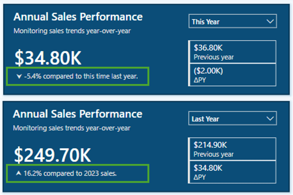
Improving Data Label Clarity

Data labels in our Power BI visuals offer users additional details, provide context, and highlight key insights. By combining the FORMAT function with descriptive text, we can create clear and easy-to-understand labels. Let’s look at an example.

This visual displays the annual total sales for each product category. To provide viewers with more information, we include a label that indicates each product’s contribution to the annual total as a percentage. Instead of presenting a percentage value without context, we enhance the label’s clarity by incorporating additional descriptive text.

This data label uses the FORMAT function and the following expression.

Product Category Totals Sales Label = 
VAR _percentage = DIVIDE([Sales Metric (CY)], [Sales Metric Annual Total])
RETURN
FORMAT(_percentage, "#0%") & " of annual sales"

We now have a clear and concise label for our visuals, allowing our viewers to quickly understand the value.

Building Dynamic Titles

Dynamic titles and subtitles in our Power BI reports can improve our report’s overall storytelling experience. They can summarize values or highlight key insights and trends, such as identifying top-performing products and year-over-year growth.

Let’s explore how to create dynamic titles and subtitles, focusing on the role of the FORMAT function in this process.

First, we need to create a measure for our visual title. The title should display the total annual sales values. Additionally, if the selected year is a previous year, the title should specify which year the annual sales data represents. To achieve this, we will use the following DAX expression.

Annual Sales Title = 
"Breaking down the " & FORMAT([Sales Metric (CY)], "$#,.00K") & 
IF(
    SELECTEDVALUE(DateTable[Year Category]) = "This Year",
    " in annual sales",
    " of annual sales in " & YEAR(MAX(DateTable[Date]))
)

The DAX measure first combines descriptive text with the formatted current year’s sales value. It then checks the selected year category from our visual slicer. If “This Year” is selected, it appends “in annual sales.” For other year selections, the title appends “of annual sales in” and explicitly includes the chosen year.

As a result, the final output will be titles such as Breaking down the $34.80K in annual sales for the current year and Breaking down the $214.90K of annual sales in 2023 when previous years are selected.

Additionally, we enhance this visual by including a dynamic subtitle that identifies top-performing products based on both annual sales and year-over-year growth.

Here is the DAX expression used to create this dynamic and informative subtitle.

Annual Sales SubTitle = 
VAR _groupByProduct = 
    ADDCOLUMNS(
        SUMMARIZE(Sales, Products[Product], "TotalSalesCY", [Sales Metric (CY)]), 
        "YOY", [Sales Metric YOY]
 )
VAR _topProductBySales = TOPN(1, _groupByProduct, [TotalSalesCY],DESC)
VAR _topProductCategoryBySales = MAXX(_topProductBySales, Products[Product])
VAR _topProductSalesValueBySales = MAXX(_topProductBySales, [TotalSalesCY])

VAR _topProductByYOY = TOPN(1, _groupByProduct, [YOY], DESC)
VAR _topProductCategoryByYOY = MAXX(_topProductByYOY, Products[Product])
VAR _topProductYOYValueByYOY = MAXX(_topProductByYOY, [YOY])

VAR _topProductCheck = _topProductCategoryBySales=_topProductCategoryByYOY

RETURN
IF(
    SELECTEDVALUE(DateTable[Year Category])="This Year",
    _topProductCategoryBySales & 
        " leads the way with " & 
        FORMAT(_topProductSalesValueBySales, "$#,.00K") & 
        " in sales" & 
        IF(_topProductCheck, " and ", ", while ") & 
        _topProductCategoryByYOY & 
        " has the highest YoY growth of " & 
        FORMAT(_topProductYOYValueByYOY, "0%"),
    _topProductCategoryBySales & 
        " led the " & 
        YEAR(MAX(DateTable[Date])) & 
        " with " & 
        FORMAT(_topProductSalesValueBySales, "$#,.00K") & 
        " in sales " & 
        IF(_topProductCheck, "and ", ", while ") & 
        _topProductCategoryByYOY & 
        " has the highest YoY growth of " &    
        FORMAT(_topProductYOYValueByYOY, "0%")
)

The measure first creates a summary table that calculates the annual sales and year-over-year (YOY) values, grouped by product category. Next, it identifies the top item for both annual sales and YOY growth, extracting the corresponding values along with the associated product category.

Total Sales

VAR _topProductBySales = TOPN(1, _groupByProduct, [TotalSalesCY],DESC)
VAR _topProductCategoryBySales = MAXX(_topProductBySales, Products[Product])
VAR _topProductSalesValueBySales = MAXX(_topProductBySales, [TotalSalesCY])

YOY Growth

VAR _topProductByYOY = TOPN(1, _groupByProduct, [YOY], DESC)
VAR _topProductCategoryByYOY = MAXX(_topProductByYOY, Products[Product])
VAR _topProductYOYValueByYOY = MAXX(_topProductByYOY, [YOY])

Next, the measure evaluates whether the top performers, determined by total sales and YoY growth, are the same.

VAR _topProductCheck = _topProductCategoryBySales=_topProductCategoryByYOY

Finally, we build the dynamic text based on the selected year and the value of _topProductCheck.

This results in subtitles like, Smartphone leads the way with $8.10K in sales and has the highest YoY growth of 37% for the current year. Alternatively, for previous, such as 2023, the subtitle reads, TV led 2023 with $70.70K in sales, while Laptop has the highest YoY growth of 106% .

BONUS: Dynamic Format Strings

Dynamic format strings are a useful preview feature in Power BI that allows us to change the formatting of a measure dynamically, depending on the context or user interaction.

One additional benefit of the dynamic format strings feature is that it preserves numeric data types. This means we can use the resulting value in situations where a numeric data type is required.

For instance, consider our report with a measure called Sales Metric (CY). Depending on the user’s selection, this measure calculates either the total annual sales or the number of annual transactions.

With dynamic format strings, if Total Sales is selected, the value is formatted as currency, and if Transactions is chosen, the value is displayed as a whole number.

With the format set to Dynamic and the format string condition defined, users can switch between the two metrics, and the values update and display dynamically.
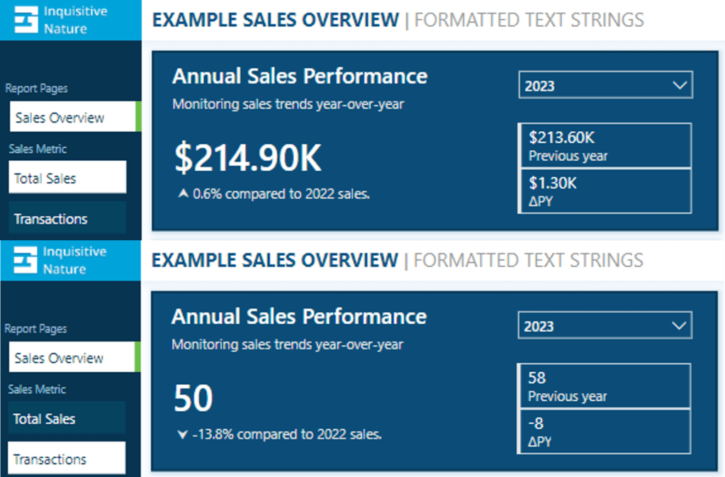
Dynamic format strings unlock a new level of customization for our Power BI reports and allow us to deliver highly polished and interactive reports.

See Create dynamic format string for measures for more details on this feature.


Wrapping Up

The FORMAT function and dynamic formatting techniques are vital tools for improving the usability, clarity, and visual appeal of our Power BI reports. These techniques allow us to create dynamic titles, develop more informative labels, and utilize dynamic format strings. By incorporating these methods, we can create interactive reports that are more engaging and user-friendly for our audience.

Continue exploring the FORMAT function and download a copy of the example file (power-bi-format-function.pbix) from my Power BI DAX Function Series: Mastering Data Analysis repository.

This dynamic repository is the perfect place to enhance your learning journey.


Thank you for reading! Stay curious, and until next time, happy learning.

And, remember, as Albert Einstein once said, “Anyone who has never made a mistake has never tried anything new.” So, don’t be afraid of making mistakes, practice makes perfect. Continuously experiment and explore new DAX functions, and challenge yourself with real-world data scenarios.

If this sparked your curiosity, keep that spark alive and check back frequently. Better yet, be sure not to miss a post by subscribing! With each new post comes an opportunity to learn something new.

Dive into DAX: Getting Started with DAX Query View


Getting Started with DAX Query View

DAX Query View in Power BI Desktop lets us interact directly with our data model using DAX queries. It provides a dedicated workspace for executing queries to explore data and validate calculations.

Clarifying the difference between DAX formulas and DAX queries here is essential, as they may become confused.

We use DAX formulas to create measures and calculated columns to extend our data model. We use DAX queries to retrieve and display existing data within our data model.

Whenever we add a field to a report or apply a filter, Power BI executes the DAX query required to retrieve and display the results. With DAX Query View, we can create and run our own DAX queries to test, explore, and validate our data models without impacting the design or outputs of our report.

Don’t just read; get hands-on and follow along with the example report provided here:

This dynamic repository is the perfect place to enhance your learning journey.


Navigating DAX Query View

We access DAX Query View within Power BI Desktop by selecting the DAX Query View icon in the left-hand Power BI view navigation.

DAX Query View contains several key components that we will become familiar with.

Command Palette: the command palette in the ribbon (or CTRL+ALT+P) provides a list of DAX query editor actions.

DAX Query Editor: this is where we write and edit our DAX queries. The editor includes features such as syntax highlighter, suggestions, and intellisense to help us construct and debug our queries.

Results Grid: when we execute a query, the data retrieved by our query appears in the results grid at the bottom of the DAX Query View window. The results grid provides instant feedback on our query or calculation outputs. When we have more than one EVALUATE statement in the Query Editor, the results grid has a dropdown we can use to switch between the results of each EVALUATE statement.

Query Tabs: located at the bottom of the DAX Query View window, different query tabs allow us to manage and navigate between multiple queries. We can create, rename, and navigate between them quickly and easily. Each tab displays a status indicator helping to identify each query’s current state (has not been run, successful, error, canceled, or running).

Data Pane: the data pane lists all the data model’s tables, columns, and measures. It provides a reference point when constructing our queries and helps us locate and include the necessary elements in our analysis. The data pane’s context menu also gives us various Quick Query options to get us started with common tasks.

For more details about the DAX Query View layout, check out the documentation: DAX Query View Layout.


Writing and Executing DAX Queries

In DAX Query View, we create and execute queries to explore and validate our data models in Power BI. DAX queries can be as simple as displaying the contents of a table to more complex, utilizing a variety of keywords.

Writing a DAX query involves using a structured syntax to retrieve data from our data model. While DAX queries provide an approach similar to SQL queries to explore our data, they are tailored specifically for working with our Power BI data model.

Every DAX query requires the EVALUATE keyword, defining the data the query will return. A DAX query at the most basic level contains a single EVALUATE statement containing a table expression.

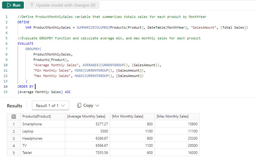
This basic query retrieves all rows from the Sales table and is a straightforward way to examine the table’s contents without adding a table visual to our report canvas.

We can build on this basic example by refining the returned data further, for example, by applying a filter to return only sales with a sales amount greater than or equal to $9,000.

Optional Keywords and Their Usage

ORDER BY

ORDER BY sorts the results of our DAX query based on one or more expressions. In addition to the expression parameter, we specify ASC (default) to sort the results in ascending order or DESC to sort in descending order.

We can continue to build on our sales query by ordering the values by descending sales amounts and ascending sales dates.

START AT

START AT is used along with the ORDER BY statement, defining the point at which the query should begin returning results.

It is important to note that the START AT arguments have a one-to-one relationship with the columns of our ORDER BY statement. This means there can be as many values in the START AT statement as in the ORDER BY statement, but not more.

We continue to build out our basic query by adding a START AT statement to take our descending list of Sales amount and return values starting at $9,500 and return the remaining results.

DEFINE

DEFINE creates one or more reusable calculated objects for the duration of our query, such as measures or variables.

The DEFINE statement and its definitions precede the EVALUATE statement of our DAX query, and the entities created within the DEFINE statement are valid for all EVALUATE statements.

Entities are created within the DEFINE statement using another set of keywords: MEASURE, VAR, COLUMN, and TABLE.

Along with the entity keyword, we must provide a name for the measure, var, table, or column definition. After the name parameter, we provide an expression that returns a table or scalar value.

MEASURE

We use theMEASURE keyword within our DEFINE statement to create a temporary local measure that persists only during the execution of our DAX query.

When we use MEASURE to define a local measure with the same name as a measure in our data model during the execution of our DAX query, the query will use the measure defined within the query rather than the measures defined in the data model. This allows us to test or troubleshoot specific calculations without modifying the data model measure.

VAR

The VAR keyword within the DEFINE statement defines a temporary variable we can use in our DAX query. Variables store the result of a DAX expression, which we can use to make our queries more straightforward to read and troubleshoot.

We use VAR to create both query variables and expression variables. When we use VAR along with our DEFINE statement, we create a query variable that exists only during the query’s execution.

We can also use VAR within an expression along with RETURN to define an expression variable local only to that specific expression.

Other keywords to be aware of within our DEFINE statement include COLUMN and TABLE. These statements allow us to create temporary calculated tables or columns that persist only during the execution of our DAX query.

Stay tuned for a follow-up blog post that will discuss the details of working with these statements and the feature-rich external tool DAX Studio.


Practical Use Cases for DAX Query View

Quick Queries

Quick Queries in DAX Query View provide a fast and easy way to start exploring aspects of our data model. They are found in the context menu when we right-click a table, column, or measure within the Data pane.

For example, we can right-click our Sales table and select Quick queries > Show top 100 rows from the context menu. Selecting this option will create a new query tab containing the DAX query resulting in the top 100 rows of our Sales table by evaluating the functions SELECTCOLUMNS() with TOPN() and using the ORDER BY statement.

We can then modify this query to tailor the results to our needs, such as only showing the RegionId, SalesDate, and Amount columns.

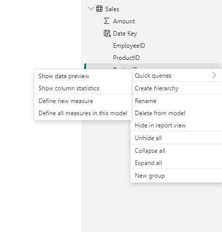
When we right-click a column and view the Quick queries, we notice the available options change and provide a Show data preview query.

Selecting this option creates a new query tab showing the distinct values of the selected column. For example, we can use this quick query in our Sales table to view our distinct Sales regions.

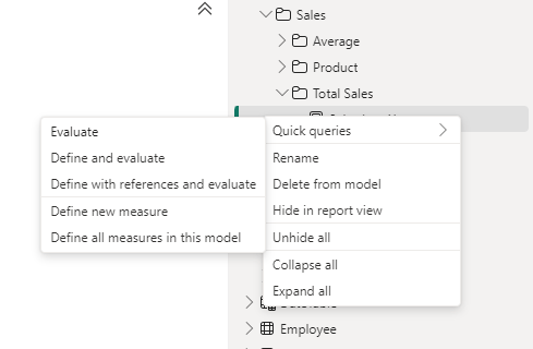
Lastly, the quick queries available within the context of measures are Evaluate, define and evaluate, and define with references and evaluate.

In our data model, we have a Sales Last Year measure. We can quickly view its value by right-clicking it and then selecting Quick queries > Evaluate.

This quick query uses SUMMARIZECOLUMNS(), which means we can quickly modify the query to add a group by column, such as Year.

We can hover over the Sales Last Year measure within the query editor window to view its DAX formula. Viewing this formula, we can see that this measure references another measure ([Total Sales]) within our data model.

We cannot view the formula for the referenced measure in the overlay. However, DAX Query View provides helpful tools to view this information. When we select a measure’s name in the query editor window, a lightbulb appears to the left.

Selecting this displays more actions available. Within the more actions menu, we choose Define with references to add a DEFINE statement to our DAX query where we can view the measure formulas. If our query already contains a DEFINE block, we will not see the lightbulb or the more actions menu.

The updated DAX query now displays the measure definitions. Note that we can get this result directly by right-clicking the measure, selecting the Define with references and evaluate quick query option.

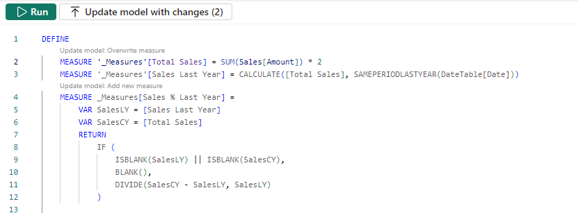
This DAX query can help test updates to the existing measures or assess the addition of new measures. For example, adding a new Sales % Last Year measure.

DAX Query View Measure Workflow

As we work with our measures in DAX Query View, it detects whether we have updated the DAX formula in an existing measure or created a new one. When a measure is updated, or a new measure is added, Query View CodeLens appears as a clickable superscript.

For example, if we update our Totals Sales measure to double it, we see the CodeLens providing us the option to update the measure within our data model. For the new Sales % Last Year measure, CodeLens gives us the option to add the new measure to the data model.

Using the measure quick queries and CodeLens assists us in streamlining our measure development workflow.

Documenting Data Models

We can also use DAX Query View to help document our data model by creating and saving queries that output model metadata.

For example, we can use the Define all measures in this model quick query to quickly create a DAX query that defines and evaluates all the measures.

In addition to viewing all the measures and their definitions in a single window, we can also use different features to understand our measures, such as using the Find option on the top ribbon to search and locate specific text (e.g. a measure’s name).

INFO Functions

DAX also includes various INFO functions that provide additional metadata on our data model to assist in documenting it. Key INFO functions include INFO.TABLES, INFO.COLUMNS, INFO.RELATIONSHIPS and INFO.MEASURES.

INFO.TABLES retrieves data about the tables in our data model, including their names, descriptions, and whether the table is hidden.

INFO.COLUMNS provides metadata for all the columns within our data model, including the column name and data type.

INFO.RELATIONSHIP provides details about the relationships between our data model tables, such as if the relationship is active, the from table and column ID, and the to table and column ID.

INFO.MEASURES lists all the measures in our data model, including their name, description, expression, and home table ID.

Since the INFO functions are just like other DAX functions, we can use them together with other DAX functions that join or summarize tables.

For example, our INFO.MEASURES function provides us with a list of all our measures. However, it just provides the home table ID, which may not be as helpful as the table name. We can create a DAX query that combines the required information from INFO.MEASURES and INFO.TABLE and returns a table with all the information we seek.

We can then review these results in the Query View results pane and save the query for future reference.

Also, check out the INFO.VIEW.COLUMNS, INFO.VIEW.MEASURES, INFO.VIEW.RELATIONSHIPS, INFO.VIEW.TABLES functions that provide similar results with the added benefit of being able to be used to define a calculated table stored and refreshed with our data model.

Optimizing Model Performance

DAX Query view also plays a role in performance optimization when we pair it with Power BI’s Performance Analyzer tool. The visuals on our report canvas get data from the data models using a DAX query. The Performance Analyzer tool lets us view this DAX query for each visual.

On the Report view, we run the Performance Analyzer by selecting the Optimize option on the ribbon and then Performance Analyzer. In the Performance Analyzer pane, we select Start recording and then Refresh visuals on the ribbon. After the visuals are refreshed, we expand the title of the visual we are interested in and choose the Run with DAX query view option to view the query in DAX Query View.

Using the Run in DAX Query View option, we review the query captured from a visual. By identifying slow-running queries and isolating their execution in DAX Query View, we can optimize DAX expressions and streamline calculations for better overall performance.


Wrapping Up

DAX Query View in Power BI Desktop creates additional possibilities for exploring our data model. Providing a dedicated workspace for writing, executing, and saving DAX queries enables us to dive deeper into our model, test calculation logic, and ensure accuracy without impacting our report or model structure.

Stay tuned for upcoming blog posts on how we can use external tools to go even further in understanding our data models using DAX queries.

To continue exploring DAX Query View, visit the following:

DAX query view – Power BI | Microsoft Learn

DAX Queries – DAX | Microsoft Learn


Thank you for reading! Stay curious, and until next time, happy learning.

And, remember, as Albert Einstein once said, “Anyone who has never made a mistake has never tried anything new.” So, don’t be afraid of making mistakes, practice makes perfect. Continuously experiment, explore, and challenge yourself with real-world scenarios.

If this sparked your curiosity, keep that spark alive and check back frequently. Better yet, be sure not to miss a post by subscribing! With each new post comes an opportunity to learn something new.

Dive into DAX: Simplify Data Models with Relationship Functions


The Basics of DAX Relationship Functions

DAX Relationship Functions are an essential part of our data modeling toolkit. These functions allow us to navigate the relationships connecting our data model tables facilitating complex calculations and deriving the insights they provide.

Relationships in our data models matter because they help maintain the integrity and consistency of our data. They connect different tables, enabling us to create insightful and dynamic reports. When creating our Power BI reports understanding these relationships becomes crucial since they dictate how data filters and aggregations are applied throughout our reports.

DAX Relationship Functions allow us to control and manipulate these relationships to suite our specific needs. Using these functions, we can perform in-depth calculations that involve multiple tables. They can be particularly useful in scenarios where we need to bring data from different sources into a single coherent view. Understanding and utilizing these functions can significantly elevate our data analysis.

For details on these functions visit the DAX Function Reference documentation.

Learn more about: DAX Relationship Functions

For those eager to start experimenting there is a Power BI report pre-loaded with the same data used in this post ready for you! So don’t just read, follow along and get hands-on with DAX in Power BI. Get a copy of the sample report here:

This dynamic repository is the perfect place to enhance your learning journey.


RELATED: Fetching Related Values

The RELATED function in DAX is designed to fetch a related value from another table. Its syntax is straightforward.

RELATED(column_name)

Here, column_name is the column from the related table that we want to retrieve. This function can be particularly useful in calculated columns when we need to access data from a lookup table in our calculations.

The RELATED function requires that a relationship exists between the two tables. Then the function can navigate the existing many-to-one relationship and fetch the specified column from the related table. In addition to an existing relationship, the RELATED function requires row context.

Our Sales table has a ProductID which is used to establish a relationship in our data model to the Products table. Let’s bring in the Product field from the Products table into our Sales table.

Product Category = RELATED(Products[Product])

We can use this DAX formula to add a new calculated column to our Sales table showing the product category corresponding to each sales record. This can help make our sales data more informative and easier to analyze, as we can now see the product category directly in the sales table.

We can also use RELATED and the existing relationship between our Sales and Regions table to filter our Sales and create an explicit United States Sales. Let’s take a look at this measure.

United States Sales = 
SUMX(
    FILTER(
        Sales, 
        RELATED(Regions[Region]) = "United States"
    ), 
    Sales[Amount]
)

This formula is much more informative and clearer than filtering directly on the RegionID field contained within the Sales table. Using RELATED within our FILTER function like this makes our measure more readable and it can immediately be identified what this measure is calculating.

The RELATED function is a powerful tool for enhancing our data models by seamlessly integrating related information. This can help us create more detailed and comprehensive reports.


RELATEDTABLE: Navigating Related Tables

The RELATEDTABLE function in DAX allows us to navigate and retrieve a table related to the current row from another table. This function can be useful when we need to summarize or perform calculations on data from a related table based on the current context. Here is its syntax.

RELATEDTABLE(table_name)

Here, table_name is the name of an existing related table that we want to retrieve. The table_name parameter cannot be an expression.

Let’s consider a scenario where we want to calculate the total sales amount for each product using the RELATEDTABLE function. Here is how we can use it to create a new calculated column in our Products table.

Total Sales by Product = 
SUMX(
    RELATEDTABLE(Sales),
    Sales[Amount]
)

In the DAX expression, we sum the Amount column from the Sales table for each product. The RELATEDTABLE function fetches all the rows from the Sales table that are related to the current product row in the Products table, and SUMX sums the Amount column for these rows.

When we use RELATEDTABLE, we can navigate and perform calculations across related tables, enhancing our ability to analyze data in a more granular and insightful way.


USERELATIONSHIP: Activating Inactive Relationships

The USERELATIONSHIP function in DAX is designed to activate an inactive relationship between tables in a data model. This is useful when a table has multiple relationships with another table, and we need to switch between these relationships for different calculations. Here is its syntax.

USERELATIONSHIP(column1, column2)

Here, column1 is the name of an existing column and typically represents the many side of the relationship to be used. The column2 is the name of an existing column and typically represents the one side or lookup side of the relationship to be used.

The USERELATIONSHIP returns no value and can only be used in functions that take a filter as argument (e.g. CALCULATE, TOTALYTD). The function uses existing relationships in the data model and cannot be used when row level security is defined for the table in which the measure is included.

Let’s take a look at a scenario where we are interested in calculating the number of employees who have left the organization based on their end dates using the USERELATIONSHIP function.

The Employee table includes each employee’s StartDate and EndDate. Each of these columns are used to establish a relationship with the DateTable in the data model. The relationship with StartDate is set to active, while the relationship with EndDate is inactive.

We can use the following DAX formula to define our Employee Separations measure.

Employees Separations USERELATIONSHIP = 
CALCULATE(
    COUNT(Employee[EmployeeID]),
    USERELATIONSHIP(Employee[EndDate], DateTable[Date]),
    NOT(ISBLANK(Employee[EndDate]))
)

This measure calculates the number of employees who have left the organization based on their EndDate by activating the inactive relationship between Employee[EndDate] and DateTable[Date] and ensuring that it only counts employees who have an EndDate.

We can better understand the power of USERELATIONSHIP by comparing these results to the results of the same measure but this time without activating the inactive relationship.

Employee Separations No USERELATIONSHIP = 
CALCULATE(
    COUNT(Employee[EmployeeID]),
    NOT(ISBLANK(Employee[EndDate]))
)

In the No USERELATIONSHIP measure we try to calculate the number of employees who left the company based on EndDate. However, we can see that without activating the relationship the active relationship is used in the context of the calculation.

Of the 9 employees that have left the organization, we can see that for 2022 the No USERELATIONSHIP measure is counting the 8 employees that started in 2022 rather than the 3 that left in 2022.


CROSSFILTER: Controlling Cross-Filtering Behavior

The CROSSFILTER function in DAX helps us manage the direction of cross-filtering between two tables in our data model. With this function we specify whether the filtering direction is one-way, both ways, or none, providing control over how data flows between our tables. This becomes useful in complex models where bidirectional filtering can lead to unintended results. Here is its syntax.

CROSSFILTER(column1, column2, direction)

The parameters column1 and column2 are similar to the parameters of USERELATIONSHIP, where column1 is the name of an existing column and typically represents the many side of the relationship and column2 is a column name and typically represents the one side of the relationship.

The direction parameter specifies the cross-filter direction to be used and must be one of the following values.

  • None – no cross-filtering occurs along this relationship
  • Both – filters on either side filters the other side
  • OneWay – filters on the one side of a relationship filter the other side. This option cannot be used with a one-to-one relationship and is not recommended for many-to-many relationships.
  • OneWay_LeftFiltersRight – filters on the side of column1 filter the side of column2. This option cannot be used with a one-to-one or many-to-one relationship.
  • OneWay_RightFiltersLeft – filters on the side of column2 filter the side of column1. This option cannot be used with a one-to-one or many-to-one relationship.

The CROSSFILTER function returns no value and can only be used within functions that take a filter as an argument (e.g. CALCULATE, TOTALYTD). When we establish relationships in our data model we define the cross-filtering direction, when we use the CROSSFILTER function it overrides this setting.

Let’s consider the scenario where we want to analyze the distinct products sold and the total sales amount by month and year. We start by creating a Distinct Product Code Count measure.

Distinct Product Code Count = 
DISTINCTCOUNT(Products[Product Code])

If we add this measure to a table visual, we will notice an issue with the count. The count is returning the total product code count, and not the intended results of the count of distinct products sold that month.

We see this because the relationship is one-to-many (Product-to-Sales) with single direction relationship (i.e. Product filters Sales). This default set up does not allow for our Sales table to filter our Product tables leading to the unintended results.

Now, we could correct this by changing the cross-filtering direction property on the Product-Sales relationship. However, this would change how filters work for all data between these two tables, which may not be a desired or an acceptable outcome.

Another solution is to utilize the power of the CROSSFILTER function. We can use this function to change how the Product-Sales relationships works within a new measure.

Distinct Product Code Count Bidirectional = 
CALCULATE(
    [Distinct Product Code Count],
    CROSSFILTER(Sales[ProductID], Products[ProductID], Both)
)

We can add this new measure to our table and see we get the expected results. This measure gathers all the sales records in the current context (e.g. Jan 2022), then filters the Product table to only related products, and finally returns a distinct count of the products sold.

This measure and the Sales Amount can now be used to analyze our sales data with details on the number of different products sold each month.

By using CROSSFILTER, we maintain control over our data relationships, ensuring our reports reflect the precise insights we need without unintended data flows. This level of control is crucial for building robust and reliable Power BI models.


Wrapping Up

DAX relationship functions are powerful tools that significantly enhance our ability to manage and analyze data in Power BI. We have explored how these essential functions empower us to connect and manipulate data and relationships within our data model. By understanding and knowing when to leverage these functions we can create dynamic, accurate, and insightful reports. Here is a quick recap of the functions.

  • RELATED simplifies data retrieval by pulling in values from a related table, making our data more informative and easier to analyze
  • RELATEDTABLE enables us to navigate and summarize related tables, providing deeper insights into our data.
  • USERELATIONSHIP gives us the flexibility to activate inactive relationships, allowing us to create more complex and context-specific calculations.
  • CROSSFILTER allows us to control the direction of cross-filtering between tables, ensuring our data flows precisely as needed.

To further explore and learn the details of these functions visit the DAX Relationship Function reference documentation.

Learn more about: DAX Relationship Functions

By adding these functions into our DAX toolkit, we enhance our ability to create flexible and robust data models that ensure our reports are both visually appealing and deeply informative and reliable.

To explore other function groups that elevate our data analysis check out the Dive into DAX series, with each post comes the opportunity to enhance your data analytics and Power BI reports.

Explore the intricate landscape of DAX in Power BI, revealing the potential to enhance your data analytics with every post. 


Thank you for reading! Stay curious, and until next time, happy learning.

And, remember, as Albert Einstein once said, “Anyone who has never made a mistake has never tried anything new.” So, don’t be afraid of making mistakes, practice makes perfect. Continuously experiment and explore new DAX functions, and challenge yourself with real-world data scenarios.

If this sparked your curiosity, keep that spark alive and check back frequently. Better yet, be sure not to miss a post by subscribing! With each new post comes an opportunity to learn something new.

Dive into DAX: Decoding Data with Power BI Logical Functions


The missing piece to decoding our data and unlocking its full potential is often the strategic application of DAX Logical Functions. These functions are pivotal in dissecting complex datasets, applying business logic, and enabling a nuanced approach to data analysis that goes beyond surface-level insights. Better understanding DAX Logical Functions allows us to create more sophisticated data models that respond with agility to analytical queries, turning abstract numbers into actionable insights.

In this post we will explore this group of functions and how we can leverage them within Power BI. We will dive in and see how we can transform our data analysis from a mere task into an insightful journey, ensuring that every decision is informed, every strategy is data-driven, and every report illuminates a path to action.


The Logical Side of DAX: Unveiling Power BI’s Brain

Diving into the logical side of DAX is where everything begins to become clear. Logical functions are the logical brain behind Power BI’s ability to make decisions. Just like we process information to decide between right and wrong, DAX logical functions sift through our data to determine truth values: true or false.

Functions such as IF, AND, OR, NOT, and TRUE/FALSE, are the building blocks for creating dynamic reports. These functions allow us to set up conditions that our data must meet, enabling a level of interaction and decision-making that is both powerful and nuanced. Whether we are determining if sales targets were hit or filtering data based on specific criteria, logical functions are our go-to tools for making sense of the numbers.

For details on these functions and many others visit the DAX Function Reference documentation.

Learn more about: DAX Logical Functions

The logical functions in DAX can go far beyond the basics. The real power happens when we start combining these functions to reflect complex business logic. Each function plays its role and when used in combination correctly we can implement complex logic scenarios.

For those eager to start experimenting there is a Power BI report pre-loaded with the same data used in this post ready for you! So don’t just read, follow along and get hands-on with DAX in Power BI. Get a copy of the sample data report here:

This dynamic repository is the perfect place to enhance your learning journey.


Understanding DAX Logical Functions: A Beginner’s Guide

When starting our journey with DAX logical functions we will begin to understand the unique role of each function within our DAX expressions. Among these functions, the IF function stands out as the decision-making cornerstone.

The IF function tests a condition, returning one result if the condition is TRUE, and another if FALSE. Here is its syntax.

IF(logical_test, value_if_true, value_if_false)

The logical_test parameter is any value or expression that can be evaluated to TRUE or FALSE, and then the value_if_true is the value that is returned if logical_test is TRUE, and the value_if_false is optional and is the value returned when logical_test is FALSE. When value_if_false is omitted, BLANK is returned when the logical_test is FALSE.

Let’s say we want to identify which sales have an amount that exceeds $5,000. To do this we can add a new calculated column to our Sales table with the following expression.

Sales Target Categorization = 
IF(
  Sales[Amount] &gt; 5000, 
  "Above Target", 
  "Below Target"
)

This expression will evaluate each sale in our Sales table, labeling each sale as either “Above Target” or “Below Target” based on the Sales[Amount].

The beauty of starting our journey with IF lies in its simplicity and versatility. While we continue to explore logical functions, it won’t be long before we encounter TRUE/FALSE.

As we saw with the IF function these values help guide our DAX expressions, they are also their own DAX function. These two functions are the DAX way of saying yes (TRUE) or no (FALSE), often used within other logical functions or conditions to express a clear binary choice.

These functions are as straightforward as they sound and do not require any parameters. When used with other functions or conditional expressions we typically use these to explicitly return TRUE or FALSE values.

For example, we can create another calculated column to check if a sale is a high value sale with an amount greater than $9,000.

High Value Sale = 
IF(
  Sales[Amount] &gt; 9000, 
  TRUE, 
  FALSE
)

This simple expression checks if the sales amount exceeds $9,000, marking each record as TRUE if so, or FALSE otherwise.

Together IF and TRUE/FALSE form the foundation of logical expressions in DAX, setting the stage for more complex decision-making analysis. Think of these functions as essential for our logical analysis, but just the beginning of what is possible.


The Gateway to DAX Logic: Exploring IF with AND, OR, and NOT

The IF function is much more than just making simple true or false distinctions; it helps us unlock the nuanced layers of our data, guiding us through the paths our analysis can take. By effectively leveraging this function we can craft detailed narratives from our datasets.

We are tasked with setting sales targets for each region. The goal is to base these targets on a percent change seen in the previous year. Depending on whether a region experienced a growth or decline, the sales target for the current year is set accordingly.

Region Specific Sales Target = 
IF(
    HASONEVALUE(Regions[Region]),
    IF(
        [Percent Change(CY-1/CY-2)] &lt; 0, 
        [Total Sales (CY-1)]*1.1, 
        [Total Sales (CY-1)]*1.2
    ),
    BLANK()
)

In this measure we make use of three other measures within our model. We calculate the total sales for the previous year (Total Sales (CY-1)), and the year before that (Total Sales (CY-2)). We then determine the percentage change between these two values.

If there is a decline (negative percent change), we set the current year’s sales target to be 10% higher than the previous year’s sales, indicating a more conservative goal. Conversely, if there was growth (positive percent change), we set the current year target 20% higher to keep the momentum going.

As we dive deeper, combining IF with functions like AND, OR, and NOT we begin to see the true flexibility of these functions in DAX. These logical operators allow us to construct more intricate conditions, tailoring our analysis to very specific scenarios.

The operator functions are used to combine multiple conditions:

  • AND returns TRUE if all conditions are true
  • OR returns TRUE if any condition is true
  • NOT returns TRUE if the condition is false

Let’s craft a measure to determine which employees are eligible for a quarterly bonus. The criterion for eligibility is twofold: the employee must have made at least one sale in the current quarter, and their average sale amount during this period must exceed the overall average sale amount.

To implement this, we first need to calculate the average sales and compare each employee’s average sale against this benchmark. Additionally, we check if the employee has sales recorded in the current quarter to qualify for the bonus.

Employee Bonus Eligibility = 
VAR CurrentQuarterStart = DATE(YEAR(TODAY()), QUARTER(TODAY()) * 3 - 2, 1)
VAR CurrentQuarterEnd = EOMONTH(DATE(YEAR(TODAY()), QUARTER(TODAY()) * 3, 1), 0)
VAR OverallAverageSale = CALCULATE(AVERAGE(Sales[Amount]), ALL(Sales))
VAR EmployeeAverageSale = CALCULATE(AVERAGE(Sales[Amount]), FILTER(Sales, Sales[SalesDate] &gt;= CurrentQuarterStart &amp;&amp; Sales[SalesDate] = CurrentQuarterStart &amp;&amp; Sales[SalesDate]  0

RETURN
IF(
    AND(HasSalesCurrentQuarter, EmployeeAverageSale &gt; OverallAverageSale),
    "Eligible for Bonus",
    "Not Eligible for Bonus"
)

In this measure we define the start and end dates of the current quarter, then we calculate the overall average sale across all data for comparison. We then determine each employee’s average sale amount and check if the employee has made any sales in the current quarter to qualify for evaluation.

If an employee has active sales and their average sale amount during the period is above the overall average, they are deemed “Eligible for Bonus”. Otherwise, they are “Not Eligible for Bonus”.

This example begins to explore how we can use IF in conjunction with AND to streamline business logic into actionable insights. These logical functions provide a robust framework for asking detailed questions about our data and receiving precise answers, allowing us to uncover the insights hidden within the numbers.


Beyond the Basics: Advanced Logical Functions in DAX

As we venture beyond the foundational logical functions we step into a world where DAX’s versatility shines, especially when dealing with complex data models in Power BI. More advanced logical functions such as SWITCH and COALESCE bring a level of clarity and efficiency that is hard to match with just basic IF statements.

SWITCH Function: Simplifying Complex Logic

The SWITCH function is a more powerful version of the IF function and is ideal for scenarios where we need to compare a single expression against multiple potential values and return one of multiple possible result expressions. This function helps us provide clarity by avoiding multiple nested IF statements. Here is its syntax.

SWITCH(expression, value, result[, value, result]...[, else])

The expression parameter is a DAX expression that returns a single scalar value and is evaluated multiple times depending on the context. The value parameter is a constant value that is matched with the results of expression, the result is any scalar expression to be evaluated if the result of expression matches the corresponding value. Finally, the else parameter is an expression to be evaluated if the result of expression does not match any value arguments.

Let’s explore. We have a scenario where we want to apply different discount rates to products based on their categories (Smartphone, Laptop, Tablet). We could achieve this by using the following expression for a new calculated column, which uses nested IFs.

Product Discount Rate (IF) = 
IF(
    Products[Product]="Smartphone", 0.10,
    IF(Products[Product]="Laptop", 0.15,
        IF(Products[Product]="Tablet", 0.20,
            0.05
        )
    )
)

Although this would achieve our goal, the use of nested if statements can make the logic of the calculated column hard to read, understand, and most importantly hard to troubleshoot.

Now, let’s see how we can improve the readability and clarity by implementing SWITCH to replace the nested IF statements.

Product Discount Rate = 
SWITCH(
    Products[Product],
    "Smartphone", 0.10,
    "Laptop", 0.15,
    "Tablet", 0.20,
    0.05
)

The expression simplifies the mapping of each Product to its corresponding discount rate and provides a default rate for categories that are not explicitly listed.

COALESCE Function: Handling Blank or Null Values

The COALESCE function offers a straightforward way to deal with BLANK values within our data, returning the first non-blank value in a list of expressions. If all expressions evaluate to BLANK, then a BLANK value is returned. Its syntax is also straightforward.

COALESCE(expression, expression[, expression]...)

Here, expression can be any DAX expression that returns a scalar value. These expressions are evaluated in the order they are passed to the COALESCE function.

When reporting on our sales data, encountering blanks can sometimes communicate the wrong message. Using COALESCE we can address this by providing a more informative value when there are no associated sales.

Product Sales = COALESCE([Total Sales], "No Sales")

With this new measure if our Total Sales measure returns a blank, for example due to filters applied in the report, COALESCE ensures this is communicated with a value of “No Sales”. This approach can be beneficial for maintaining meaningful communication in our reports. It ensures that our viewers understand the lack of sales being reported, rather than interpreting a blank space as missing or erroneous data.

These logical functions enrich our DAX toolkit, enabling more elegant solutions to complex problems. By efficiently managing multiple conditions and safeguarding against potential errors, SWITCH and COALESCE not only optimize our Power BI models but also enhance our ability to extract meaningful insights from our data.

With these functions, our journey into DAX’s logical capabilities becomes even more exciting, revealing the depth and breadth of analysis we can achieve. Let’s continue to unlock the potential within our data, leveraging these tools to craft insightful, dynamic reports.


Logical Comparisons and Conditions: Crafting Complex DAX Logic

Delving deeper into DAX, we encounter scenarios that demand a blend of logical comparisons and conditions. This complexity arises from weaving together multiple criteria to craft intricate logic that precisely targets our analytical goals.

We touched on logical operators briefly in a previous section, the AND, OR, and NOT functions are crucial for building complex logical structures. Let’s continue to dive deeper into these with some more hands-on and practical examples.

Multi-Condition Sales Analysis

We want to identify and count the number Sales transactions that meet specific criteria: sales above a threshold and within a particular region. To achieve this, we create a new measure using the AND operator to count the rows in our sales table that meet our criteria.

High Value Sales in US (Count) = 
COUNTROWS(
    FILTER(
        Sales,
        AND(
            Sales[Amount] &gt; 5500,
            RELATED(Regions[Region]) = "United States"
        )
    )
)

This measure filters our Sales table to sales that have an amount greater than our threshold of $5,500 and have a sales region of United States.

Excluding Specific Conditions

We need to calculate total year-to-date sales while excluding sales from a particular region or below a certain amount. We can leverage the NOT function to achieve this.

Sales Excluding Asia and Low Values = 
CALCULATE(
    SUM(Sales[Amount]),
    AND(
        NOT(Sales[RegionID] = 3), // RegionID=3 (Asia)
        Sales[Amount] &gt; 5500
    ),
    Sales[IsCurrentYear]=TRUE()
)

This measure calculates the sum of the sales amount that are not within our Asia sales region and are above $5,500. Using NOT we exclude sales from the Asia region and we us the AND function to also impose the minimum sales amount threshold.

Special Incentive Qualifying Sales

Our goal is to identify sales transactions eligible for a special incentive based on multiple criteria: sales amount, region, employee involvement, and a temporal aspect of the sales data. Here is how we can achieve this.

Special Incentive Qualifying Sales = 
CALCULATE(
    SUM(Sales[Amount]),
    OR(
        Sales[Amount] &gt; 7500,
        Sales[RegionID] = 2
    ),
    NOT(
        Sales[EmployeeID] = 4
    ),
    Sales[IsCurrentYear] = TRUE()
)

The OR function is used to include sales transactions that either exceed $7,500 or are made in Europe (RegionID = 2) and the NOT function excludes transaction made by an employee (EmployeeID = 4), who is a manager and exempt from the incentive program. The final condition is that the sale occurred in the current year.

The new measure combines logical tests to filter our sales data, identifying the specific transactions that qualify for a special incentive under detailed conditions.

By leveraging DAX’s logical functions to construct complex conditional logic, we can precisely target specific segments of our data, uncover nuanced insights, and tailor our analysis to meet specific business needs. These examples showcase just the beginning of what is possible when we combine logical functions in creative ways, highlighting DAX’s robustness and flexibly in tackling intricate data challenges.


Wrapping Up: From Logic to Action

Our journey through the world of DAX logical functions underscores their transformative power within our data analysis. By harnessing IF, SWITCH, AND, OR, and more, we’ve seen how data can be sculpted into actionable insights, guiding strategic decisions with precision. To explore other DAX Logical Functions or get more details visit the DAX Function Reference.

Learn more about: DAX Logical Functions

Logical reasoning in data analysis is fundamental. It allows us to uncover hidden patterns and respond to business needs effectively, demonstrating that the true value of data lies in its interpretation and application. DAX logical functions are the keys to unlocking this potential, offering clarity and direction in our sea of numbers.

As we continue to delve deeper into DAX and Power BI, let the insights derived from logical functions inspire action and drive decision-making. To explore other functions groups that elevate our data analysis check out the Dive into DAX series, with each post comes the opportunity to enhance your data analytics and Power BI reports.

Explore the intricate landscape of DAX in Power BI, revealing the potential to enhance your data analytics with every post. 


Thank you for reading! Stay curious, and until next time, happy learning.

And, remember, as Albert Einstein once said, “Anyone who has never made a mistake has never tried anything new.” So, don’t be afraid of making mistakes, practice makes perfect. Continuously experiment and explore new DAX functions, and challenge yourself with real-world data scenarios.

If this sparked your curiosity, keep that spark alive and check back frequently. Better yet, be sure not to miss a post by subscribing! With each new post comes an opportunity to learn something new.

Dive into DAX: Elevated Insights with Information Functions


In data analytics effectively navigating, understanding, and interpreting our data can be the difference between data-driven insights and being lost in a sea of data. In this post we will focus on a subset of DAX functions that help us explore our data – the Information Functions.

These functions are our key to unlocking deeper insights, ensuring data integrity, and enhancing the interactivity of our reports. Let’s embark on a journey to not only elevate our understanding of Power BI and DAX but also to harness the full potential of our data.

The Role of Information Functions in DAX

Information functions play a crucial role in DAX. They are like the detective of our Power BI data analysis, helping us identify data types, understand relationships, handling errors, and much more. Whether we are checking for blank values, understanding the data type, or handling various data scenarios, information functions are our go-to tools.

Diving deep into information functions goes beyond today’s problems and help prepare for tomorrow’s challenges. Mastering these functions enables us to clean and transform our data efficiently, making our analytics more reliable and our insights more accurate. It empowers us to build robust models that stand the test of time and data volatility.

In our exploration through the world of DAX Information Functions, we will explore how these functions work, why they are important, and how we can use them to unlock the full potential of our data. Ready to dive in?

For those of you eager to start experimenting there is a Power BI report pre-loaded with the same data used in this post ready for you. So don’t just read, follow along and get hands-on with DAX in Power BI. Get a copy of the sample data file here:

This dynamic repository is the perfect place to enhance your learning journey.


The Heartbeat of Our Data: Understanding ISBLANK and ISEMPTY

In data analysis knowing when our data is missing, or blank is key. The ISBLANK and ISEMPTY functions in DAX help us identify missing or incomplete data.

ISBLANK is our go-to tool to identify voids within our data. We can use this function to locate and handle this missing data either to report on it or to manage it, so it does not unintentionally impact our analysis. The syntax is straightforward.

ISBLANK(value)

Here, value is the value or expression we want to check.

Let’s use this function to create a new calculated column to check if our sales amount is blank. This calculated column can then be used to flag and identify these records with missing data, and ensure they are accounted for in our analysis.

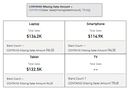
MissingSalesAmount = ISBLANK(Sales[Amount])

We can now use this calculated column to provide a bit more context to card visuals showing our total sales for each of our products.

In this example we can see the total sales for each product category. However, if we only show the total sales value it could lead our viewers to believe that the TV category has no sales. By adding a count of TV Sales records that have a blank sales amount we can inform our viewers this is not the case and that there is an underlying data issue.

While ISBLANK focuses on the individual values, ISEMPTY takes a step back to consider the table as a whole. We can use this function to check whether the table we pass to this DAX expression contains data. Its syntax is also simple.

ISEMPTY(table_expression)

The table_expression parameter can be a table reference or a DAX expression that returns a table. ISEMPTY will return a value of true if the table has no rows, otherwise it returns false.

Let’s use ISEMPTY in combination with ISBLANK to check if any of our sales records have a missing or blank employee Id. Then we can use this information, to display the count of records (if any) and the total sales value of these records.

In this example we see that Sales with No EmployeeId returns a value of false, indicating that the table resulting from filtering our sales records to sales with a blank employee Id is not empty and contains records. We can then also make use of this function to help display the total sales of these records and a count.

These two functions are the tools to use when investigating our datasets for potentially incomplete data. ISBLANK can help us identify rows that need attention or consideration in our analysis and ISEMPTY helps validate if a subset of data exists in our datasets. To effectively utilize these two functions, it is important to remember their differences. Remember ISBLANK checks if an individual value is missing data, while ISEMPTY examines if a table contains rows.


The Data Type Detectives: ISTEXT, ISNONTEXT, ISLOGICAL and ISNUMBER

In the world of data, not every value is as it seems and that is where this set of helpful DAX expressions come into play. These functions help identify the data types of the data we use within our analysis.

All of these functions follow the same syntax.

ISTEXT(value)
ISNONTEXT(value)
ISLOGICAL(value)
ISNUMBER(value)

Each function checks the value and returns true or false. We will use a series of values to explore how each of these functions work. To do this we will create a new table which uses each of these functions to check the values: TRUE(), 1.5, “String”, “1.5”, and BLANK(). Here is how we can do it.

TestValues = 
VAR _logical = TRUE()
VAR _number = 1.5
VAR _text = "String"
VAR _stringNumber = "1.5"

VAR _testTable =
{
   ("ISLOGICAL", ISLOGICAL(_logical), ISLOGICAL(_number), ISLOGICAL(_text), ISLOGICAL(_stringNumber), ISLOGICAL(BLANK())),
   ("ISNUMBER", ISNUMBER(_logical), ISNUMBER(_number), ISNUMBER(_text), ISNUMBER(_stringNumber), ISNUMBER(BLANK())),
   ("ISTEXT", ISTEXT(_logical), ISTEXT(_number), ISTEXT(_text), ISTEXT(_stringNumber), ISTEXT(BLANK())),
   ("ISNONTEXT", ISNONTEXT(_logical), ISNONTEXT(_number), ISNONTEXT(_text), ISNONTEXT(_stringNumber), ISNONTEXT(BLANK()))
}

RETURN
SELECTCOLUMNS(
   _testTable,
   "Function", [Value1],
   "Test Value: TRUE", [Value2],
   "Test Value: 1.5", [Value3],
   "Test Value: String", [Value4],
   "Test Value: '1.5'", [Value5],
   "Test Value: BLANK", [Value6]
)

An then we can add a table visual to our report to see the results and better understand how each function treats our test values.

The power of these functions lies in their simplicity, the clarity they can bring to our data preparation process, and their ability to be used in combination with other expressions to handle complex data scenarios.

DAX offers a number of other functions that are similar to the ones explored here such as ISEVEN, ISERROR, and ISAFTER. Visit the DAX reference guide for all the details.

Learn more about: DAX Information Functions

A common issue we can run into in our analysis is assuming data types based on a value’s appearance or context, leading to errors in our analysis. Mistakenly performing a numerical operation on a text field that appear numeric can easily throw our results into disarray. Using these functions early in our process to understand our data paves the way for clean, error-free data processing.


The Art of Data Discovery: CONTAINS & CONTAINSSTRING

When diving into our data, pinpointing the information we need can be a daunting task. This is where DAX steps in and provides us CONTAINS and CONTAINSSTRING. These functions help us uncover the specifics hidden within our data.

CONTAINS can help us identify whether a table contains a row that matches our criteria. Its syntax is as follows.

CONTAINS(table, columnName, value[, columnName, value]...)

The table parameter can be any DAX expression that returns a table of data, columnName is the name of an existing column, and value is any DAX expression that returns a scalar value that we are searching for in columnName.

CONTAINS will return a value of true if each specified value can be found in the corresponding columnName (i.e. columnName contains value), otherwise it will return false.

In our previous ISBLANK example we created a Blank Count measure to help us identify how many sales records for our product categories are missing sales amounts.

Blank Count = 
COUNTROWS(
   FILTER(Sales, Sales[MissingSalesAmount]=true)
)

Now, if we are interested in knowing just if there are missing sales amounts, we could update this expression to return true if COUNTROWS returns a value greater than 0, however this is where we can use CONTAINS to create a more effective measure.

Missing Sales Amount = 
CONTAINS(Sales, Sales[MissingSalesAmount], TRUE())

CONTAINS can be a helpful tool, however, it is essential to distinguish when it is the best tool for the task versus when an alternative might offer a more streamlined approach. Alternatives to consider include functions such as IN, FILTER, or TREATAS depending on the need.

For example, CONTAINS can be used to establish a virtual relationship between our data model tables, but functions such as TREATAS may provide better efficiency and clarity. For details on this function and its use check out this post for an in-depth dive into DAX Table Manipulation Functions.

Discover how to Reshape, Manipulate, and Transform your data into dynamic insights.

For searches based on textual content, CONTAINSTRING is our go to tool. It specializes in revealing rows where text columns contain specific substrings. The syntax is straightforward.

CONTAINSSTRING(within_text, find_text)

The within_text parameter is the text we want to search for the text passed to the find_text parameter. This function will return a value of true if find_text is found, otherwise it will return false.

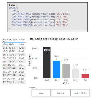
We can use CONTAINSSTRING to dissect our Product Code and enrich our dataset by adding a calculated column containing a user-friendly color value of the product. Here is how.

Color = SWITCH(
    TRUE(),
    CONTAINSSTRING(Products[Product Code], "BK"), "Black",
    CONTAINSSTRING(Products[Product Code], "rd"), "Red",
    CONTAINSSTRING(Products[Product Code], "GR"), "Gray",
    CONTAINSSTRING(Products[Product Code], "SL"), "Silver",
    CONTAINSSTRING(Products[Product Code], "BL"), "Blue"
)

This new calculated column provides us the color of each product that we can use in a slicer, or we can visualize our totals sales by the product color.

CONSTAINSSTRING is case-insensitive, as shown in the red color statement above. When we require case-sensitivity CONSTAINSSTRINGEXACT provides us this functionality.

CONTAINSSTRING just begins to scratch the surface of the DAX functions available to use for in-depth textual analysis, to continue exploring visit this post that focuses solely on DAX Text Functions.

Stringing Along with DAX: Dive Deep into Text Expressions

By leveraging CONTAINS and CONTAINSTRING – alongside understanding when to employ their alternatives – we are equipped with the tools required for precise data discovery within our data analysis.


Deciphering Data Relationships: ISFILTERED & ISCROSSFILTERED

Understanding the dynamics of data relationships is critical for effective analysis. In the world of DAX, there are two functions we commonly turn to that guide us through the relationship network of our datasets: ISFILTERED and ISCROSSFILTERED. These functions provide insights into how filters are applied within our data model, offering a deeper understanding of the context in which our data operates.

ISFILTERED offers a window into the filtering status of a table or column, allowing us to determine whether a filter has been applied directly to that table or column. This insight is valuable for creating responsive measures that adjust based on user selections or filter context. The syntax is as follows.

ISFILTERED(tableName_or_columnName)

A column or table is filtered directly when a filter is applied to any column of tableName or specifically to columnName.

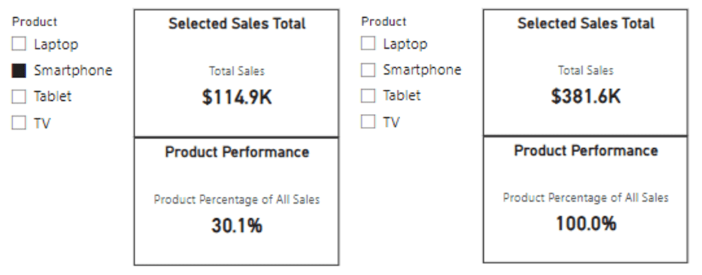
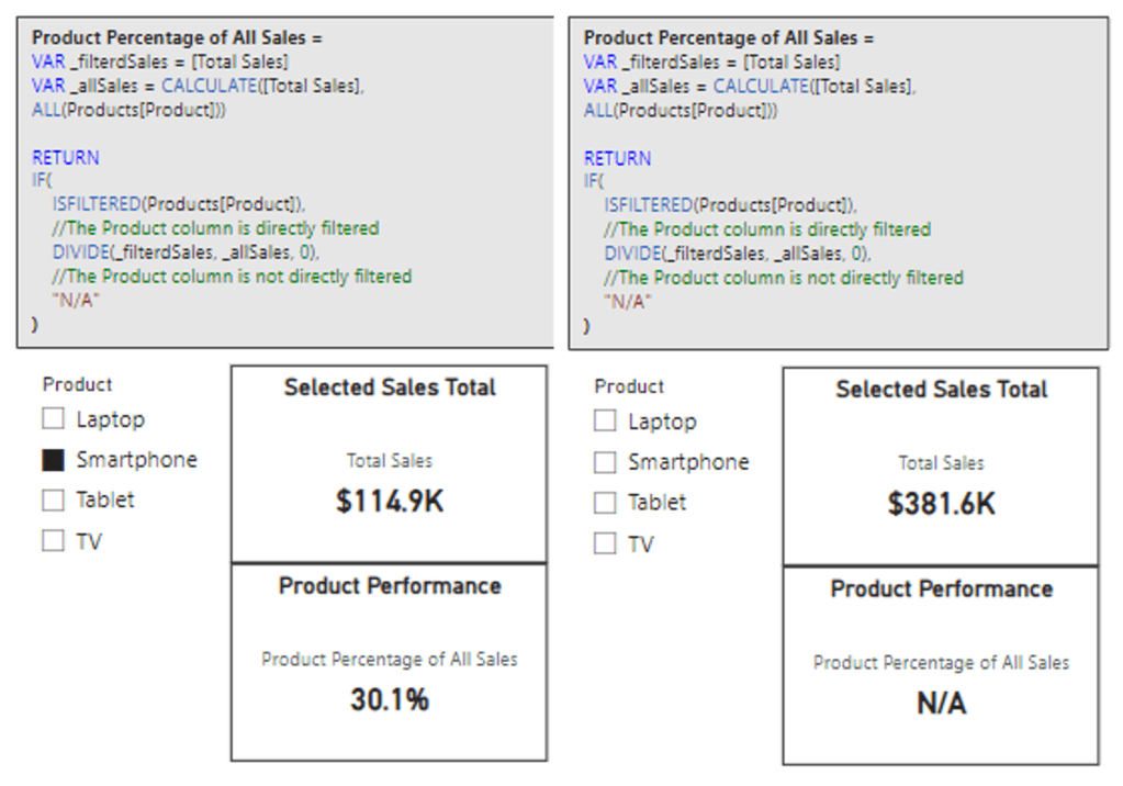
Let’s create a dynamic measure that leverages ISFILTERED and reacts to user selections. In our data model we have a measure that calculates the product sales percentage of our overall total sales. This measure is defined by the following expression.

Product Percentage of All Sales = 
VAR _filterdSales = [Total Sales]
VAR _allSales = CALCULATE([Total Sales], ALL(Products[Product]))

RETURN
DIVIDE(_filterdSales, _allSales, 0)

We can see this measure displays the percentage of sales for the selected product. However, when no product is selected it displays 100%, although this is expected and correct, we would rather not display the percentage calculation when there is no product selected in our slicer.

This is a perfect case to leverage ISFILTERED to first check if our Products[Product] column is filtered, and if so, we can display the calculation, and if not, we will display “N/A”. We will update the measure’s definition to the following.

Product Percentage of All Sales = 
VAR _filterdSales = [Total Sales]
VAR _allSales = CALCULATE([Total Sales], ALL(Products[Product]))

RETURN
IF(
    ISFILTERED(Products[Product]),
    //The Product column is directly filtered
    DIVIDE(_filterdSales, _allSales, 0),
    //The Product column is not directly filtered
    "N/A"
)

And here are the updated results, we can now see when no product is selected in the slicer the measure displays “N/A”, and when the user selects a product, the measure displays the calculated percentage.

While ISFILTERED focuses on direct filter application, understanding the impact of cross-filtering, or how filters on one table affect another related table, is just as essential in our analysis. ISCROSSFILTERED goes beyond ISFILTERED and helps us identify if a table or column has been filtered directly or indirectly. Here’s its syntax.

ISCROSSFILTERED(tableName_or_columnName)

ISCROSSFILTERED will return a value of true when the specified table or column is cross-filtered. The table or column is cross-filtered when a filter is applied to columnName, any column of tableName, or any column of a related table.

Let’s explore ISCROSSFILTERED and how it differs from ISFILTERED with a new measure similar to the one we just created. We define the new measure as the following.

Product Percentage of All Sales CROSSFILTER = 
VAR _filterdSales = [Total Sales]
VAR _allSales = CALCULATE([Total Sales], ALL(Sales))

RETURN
IF(
    ISCROSSFILTERED(Sales),
    //Sales table is cross-filtered
    DIVIDE(_filterdSales, _allSales, 0),
    //The Sales table is not cross-filterd
    "N/A"
)

In this measure we utilize ISCROSSFILTERED to check if our Sales table is cross-filtered, and if it is we calculate the proportion of filtered sales to all sales, otherwise the expression returns “N/A”. With this measure we can gain a nuanced view of product performance within the broader sales context.

When our Sales table is only filtered by our Product slicer, we see that the ISFILTERED measure and the ISCROSSFILTERED measure return the same value (below on the left). This is because as before the column Products[Product] is directly filtered by our Product slicer, so the ISFILTERED measure carries out the calculation and returns the percentage.

But also, since our data model has a relationship between our Product and Sales table, the selection of a product in the slicer indirectly filters, or cross-filters, our Sales table leading to our CROSSFILTER measure returning the same value.

We start to see the difference in these functions when we start to incorporate other slicers, such as our region slicer. In the middle image, we can see if no product is selected our Product Performance card display “N/A”, because our Products[Product] column is not being directly filtered.

However, the Sales Performance card that uses our CROSSFILTER measure is dynamically updated to now display the percentage of sales associated with the selected region. Again, this is because our data model has a relationship between our Region and Sales table, so the selection of a region is cross-filtering our sales data.

Lastly, we can see both measures in action when a Product and Region are selected (below on the right).

Using ISFILTERED, we can create reports that dynamically adjust to user interactions, offering tailored insights based on specific filters. ISCROSSFILTERED takes this a step further by allowing us to understand and leverage the nuances of cross-filtering impacts within our data, enabling an even more sophisticated analytical approach.

Applying these two functions within our reports allows us to enhance data model interactivity and depth of analysis. This helps us ensure our reports respond intelligently to user interactions and reflect the complex interdependencies within our data.


Wrapping Up

Compared to other function groups DAX Information Functions may be overlooked, however these functions can hold the key to unlocking insights, providing a deeper understanding of our data’s structure, quality, and context. Effectively leveraging these functions can elevate our data analysis and integrating them with other DAX function categories can lead to the creation of dynamic and insightful solutions.

As we continue to explore the synergies between different DAX functions, we pave the way for innovative solutions that can transform raw data into meaningful stories and actionable insights. For more details on Information Functions and other DAX Functions visit the DAX Reference documentation.

Learn more about: DAX Functions


Thank you for reading! Stay curious, and until next time, happy learning.

And, remember, as Albert Einstein once said, “Anyone who has never made a mistake has never tried anything new.” So, don’t be afraid of making mistakes, practice makes perfect. Continuously experiment and explore new DAX functions, and challenge yourself with real-world data scenarios.

If this sparked your curiosity, keep that spark alive and check back frequently. Better yet, be sure not to miss a post by subscribing! With each new post comes an opportunity to learn something new.