Mastering DAX Text Expressions: Making Sense of Your Data One String at a Time


Ever felt like your data was whispering secrets just beyond your grasp? Dive into the world of DAX Text Functions and turn those whispers into powerful narratives. Unlock stories hidden within text strings, and let your data weave tales previously untold.


Introduction to DAX Text Functions

We live in a world that’s overflowing with data. But let’s remember: data can be so much more than just numbers on a spreadsheet. It can be the letters we string together, and the words we read. Get ready to explore the exciting world of DAX Text Functions!

If you have ever worked with Power BI, you are likely familiar with DAX or Data Analysis Expressions. If you are new to Power BI and DAX check out these blog posts to get started:

Row Context — What it is, When is it available, and its Implications

Iterator Functions — What they are and What they do

DAX is the backbone that brings structure and meaning to the data we work with in Power BI. Especially when we are dealing with textual data, DAX stands out with its comprehensive set of functions dedicated just for this purpose.

So whether you’re an experienced data analyst or a beginner just starting your journey, you have landed on the right page. Prepare to explore the depth and breadth of DAX Text Functions. This is going to be a deep dive covering various functions, their syntax, and plenty of of examples!

For those of you eager to start experimenting there is a Power BI report loaded with the sample data used in this post ready for you. So don’t just read, dive in and get hands-on with DAX Functions in Power BI. Check out it here:

This dynamic repository is the perfect place to enhance your learning journey.


LEFT, RIGHT, & MID — The Text Extractors

Starting with the basics, LEFT, RIGHT, and MID. Their primary role is to provide tools for selectively snipping portions of text, enabling focused data extraction. Let’s go a little deeper and explore their nuances.

LEFT Function: As the name subtly suggests, the LEFT function fetches a specific number of characters from the start, or leftmost part, of a given text string.

The syntax is as simple as:

LEFT(text, number_of_characters)

Here, text is the text string containing the characters you want to extract, and number_of_characters is an optional parameter that indicates the number of characters you want to extract. It defaults to a value of 1 if a value is not provided.

For more details see:

Learn more about: LEFT

RIGHT Function: The RIGHT function, mirrors the functionality of LEFT and aims to extract the characters from the end of a string, or the rightmost part.

The syntax is the same as we saw for LEFT:

RIGHT(text, number_of_characters)

For more details see:

Learn more about: RIGHT

MID Function: Now we have the MID function. This is the bridge between LEFT and RIGHT that doesn’t restrict you to the start or end of the text string of interest. MID enables you to pinpoint a starting position and then extract a specific number of characters from there.

The syntax is as follows:

MID(text, start_number, number_of_characters)

Here, text is the text string containing the characters you want to extract, start_number is the position of the first character you want to extract (positions in the string start at 1), and number_of_characters is the number of characters you want to extract.

For more details see:

Learn more about: MID

Practical Examples: Diving Deeper with the Text Extractors

Let’s dive deeper with some examples. Let’s say we have a Product Code column within our Product Table. The Product Code takes the form of product_abbreviation-product_num-color_code for example, SM-5933-BK.

We will first extract the first two characters using LEFT, these represent the product abbreviation. We can create a calculated column in the products table using the following expression:

Product Abbrev = LEFT(Products[Product Code], 2)

Next, let’s use RIGHT to extract the last two characters which represent the color code of the product. We will add another calculated column to the products table using the following:

Product Color = RIGHT(Products[Product Code], 2)

Lastly, to pinpoint the unique product number which is nestled in the middle we will use MID. We add another calculated column to the products table using this expression:

Product Number = MID(Products[Product Code], 4, 4)

Together, these three functions form the cornerstone of text extraction. However, they can sometimes stumble when there are unexpected text patterns. Take, for instance, the last row shown below for Product Code TBL-57148-BLK.

You might have noticed that the example expressions above may not always extract the intended values due to their reliance on hardcoded positions and number of characters. This highlights the importance of flexible and dynamic text extraction methods.

Enter FIND and SEARCH! As we venture further into this post, we will uncover how these functions can provide much-needed flexibility to our extractions, making them adaptable to varying text lengths and structures. So, while the trio of LEFT, RIGHT, and MID are foundational, there is a broader horizon of DAX Text Functions to explore.

So, don’t halt your DAX journey here; continue reading and discover the expanded universe of text manipulation tools. Dive in, and let’s continue to elevate your DAX skills.


FIND & SEARCH — Navigators of the Text Terrain

In the landscape of DAX Text Functions, FIND and SEARCH stand out as exceptional navigators, aiding you in locating a substring within another text string. Yet, despite their apparent similarities, they come with clear distinctions that could greatly impact your results.

FIND Function: the detail-oriented one of the two functions. It is precise, and is case-sensitive. So, when using FIND, ensure you embrace the details and match the exact case of the text string you are seeking.

The syntax of FIND is:

FIND(find_text, within_text[, [start_number][, NotFoundValue]])

Here, find_text is the text string you are seeking, you can use empty double quotes "" to match the first character of within_text. Speaking of, within_text is the text string containing the text you want to find.

The other parameters are optional, start_number is the position in within_text to start the seeking and defaults to 1 meaning the start of within_text. Lastly, NotFoundValue although optional is highly recommended and represents the value the function will use when find_text is not found in within_text, typical values include 0, -1.

For more details see:

Learn more about: FIND

SEARCH Function: SEARCH is the more laid-back of the two functions. It is adaptable and does not account for case, whether it’s upper case, lower case or a mix SEARCH will find the text you are looking for.

The syntax for SEARCH is as follows:

SEARCH(find_text, within_text[, [start_number][, NotFoundValue]])

SEARCH operates using the same parameters as FIND, which can facilitate a streamlined approach when having to switch between them.

For more details see:

Learn more about: SEARCH

Practical Examples: Amplifying Flexibility

When combined with LEFT, RIGHT, or MID the potential of FIND and SEARCH multiplies, allowing for dynamic text extraction. Let’s consider the problematic Product Code TBL-57148-BLK again.

We started by extracting the product abbreviation with the following expression:

Product Abbrev = LEFT(Products[Product Code], 2)

This works well when all the product codes start with a two-letter abbreviation. But what if they don’t? The fixed number of characters to extract might yield undesirable results. Let’s use FIND to add some much-needed flexibility to this expression.

We know that the product abbreviation is all the characters before the first hyphen. To determine the position of the the first hyphen we can use:

First Hyphen = FIND("-", Products[Product Code])

For TBL-57148-BLK this will return a value of 4. We can then use this position to update our expression to dynamically extract the product abbreviation.

Product Abbrev Dynamic = 
LEFT(
  Products[Product Code], 
  FIND("-", Products[Product Code]) - 1
)

Next, let’s add some adaptability to our Product Color expression to handle when the color code may contain more than two characters. We started with the following expression:

Product Color = RIGHT(Products[Product Code], 2)

This expression assumes that all product color codes are consistently placed at the end and always two characters. However, if there are variations in the length (e.g. TBL-57148-BLK) this method might not be foolproof. To introduce some adaptability, let’s utilize SEARCH.

To determine the position of the last hyphen, since the color code will always be all the characters following this we can use:

Last Hyphen =
SEARCH (
    "-",
    Products[Product Code],
    FIND ( "-", Products[Product Code] ) + 1
)

Here, for the start_number we use the same FIND expression that we did to locate the first hyphen and then add 1 to the position to start the search for the second.

With this position, we can update our Product Color function to account for potential variations:

Product Color Dynamic =
VAR _firstHyphenPosition =
    FIND (
        "-",
        Products[Product Code]
    )
VAR _lastHyphenPosition =
    SEARCH (
        "-",
        Products[Product Code],
        _firstHyphenPosition + 1
    )
RETURN
    RIGHT (
        Products[Product Code],
        LEN ( Products[Product Code] ) - _lastHyphenPosition
    )

The updated calculated column finds the position of the first hyphen, and then uses this position to search for the position of the last hyphen. Once we know the position, we can use this position and the length of the string to determine the number of characters needed to extract the color code ( LEN(Products[Product Code]) - _lastHyphenPosition).

Through the use of FIND, SEARCH, and RIGHT, the DAX text extraction becomes more adaptable, and handles even unexpected product code formats with ease.

Similarly, we can update the the Product Number expression to:

Product Number Dynamic =
VAR _firstHyphenPosition =
    FIND (
        "-",
        Products[Product Code]
    )
VAR _lastHyphenPosition =
    SEARCH (
        "-",
        Products[Product Code],
        _firstHyphenPosition + 1
    )
VAR _productNumberLength = _lastHyphenPosition - _firstHyphenPosition - 1
RETURN
    MID (
        Products[Product Code],
        _firstHyphenPosition + 1,
        _productNumberLength
    )

Through these examples we have highlighted how to build upon the basics of LEFT, RIGHT, and MID by amplifying their flexibility through the use of FIND and SEARCH.

Practical Examples: Demonstrating Distinct Characteristics

When it comes to locating specific strings within a text string, both FIND and SEARCH offer a helping hand. But, as is often the case with DAX, the devil is in the details. While they seem quite similar at a glance, a deeper exploration uncovers unique traits that set them apart. What’s main difference? Case sensitivity.

Let’s explore this by comparing the results of the following expressions:

Position with FIND = FIND("rd", Products[Product Code], 1, -1)
Position with SEARCH = SEARCH("rd", Products[Product Code], -1)

In these example DAX formulas we can see the key difference between FIND and SEARCH. Both calculated columns are looking for “rd” within the Product Code. However, for SM-7818-RD we see FIND does not identify “rd” as a match whereas SEARCH does identify “rd” as a match starting at position 9.

Both of these functions are essential tools in your DAX toolbox, your choice between them will hinge on whether case sensitivity is a factor in your data analysis needs.

By mastering the combination of these text functions, you not only enhance text extraction but also pave the way to advanced text processing with DAX. The intricate synergy of FIND and SEARCH with other functions like LEFT, RIGHT, and MID showcases DAX’s textual data processing potential. Keep reading, as we journey further into more complex and fascinating DAX functions!


CONCATENATE & COMBINEVALUES — Craftsmen of Cohesion

While both CONCATENATE and COMBINEVALUES serve the primary purpose of stringing texts together, they achieve this with unique characteristics. CONCATENATE is the timeless classic, merging two strings with ease, while COMBINEVALUES adds modern finesse by introducing delimiters.

CONCATENATE Function: is designed to merge two text strings, with a syntax as simple as the concept.

CONCATENATE(text1, text2)

The first text string you want to merge is represented by text1, and the second text string to be merged is represented by text2. The text strings can include text, numbers, or you can use a column references.

For more details see:

Learn more about: CONCATENATE

COMBINEVALUES Function: combines text strings while also integrating a specified delimiter between them, adding some versatility when needed. The syntax is as follows:

COMBINEVALUES(delimiter, expression, expression[, expression]...)

The character or set of characters you wish to use as a separator is denoted by delimiter. The expression parameters are the DAX expressions whose value will be joined into the single string.

For more details see:

Learn more about: COMBINEVALUES

Practical Examples: Illuminating Their Craft

Let’s put these functions to use and examine some real-world scenarios.

Let’s say we need to create a new Product Label column in the Products table. The label should consist of the product abbreviation directly followed by the product number. We can achieve this using the previously created columns Product Abbrev Dynamic and Product Number Dynamic along with CONCATENATE. The expression for the new column would look like this:

Product Label =
CONCATENATE (
    Products[Product Abbrev Dynamic],
    Products[Product Number Dynamic]
)

The expression merges the dynamically determined product abbreviation and product number.

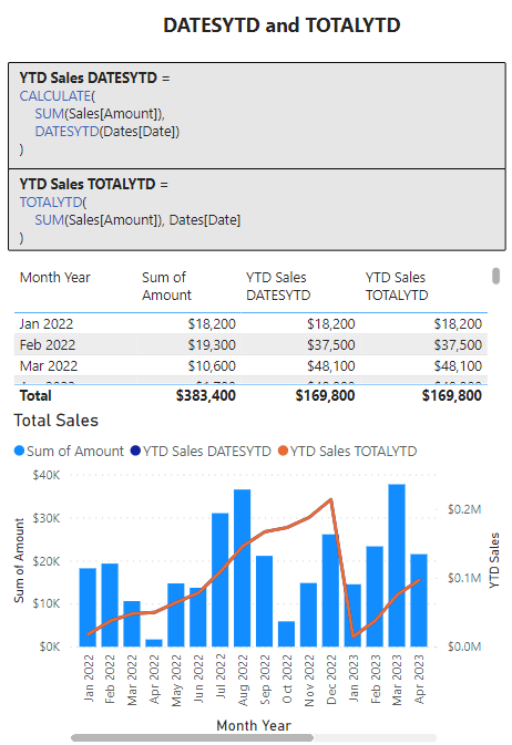
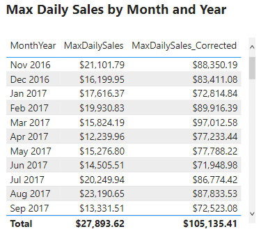
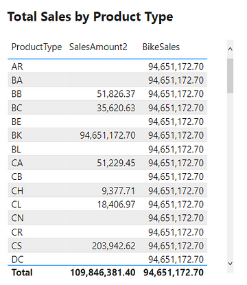
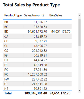
Now, let’s change it up a bit and work with creating a new measure with COMBINEVALUES. Say, we need a page of the report specific to the current year’s sales and we want to create a page title that provides the current year and the YTD sales value. Additionally, we want to avoid hardcoding the current year value and the YTD sales figure because these will continually change and would require continual updating. We can use COMBINEVALUES to meet this requirement, and the expression would look like this:

Yearly Page Title =
COMBINEVALUES (
    " ",
    YEAR (TODAY ()),
    "- Year to date sales:",
    FORMAT ([YTD Sales TOTALYTD], "Currency")
)

This measure, dynamically generates the title text by combining the current year (Year(TODAY())), the text string “- Year to date sales:”, followed by a YTD measure ([YTD Sales TOTALYTD]).

The [YTD Sales TOTALYTD] measure uses a another set of powerful DAX functions: Time Intelligence functions. For details on the creation of the [YTD Sales TOTALYTD] along with other Time Intelligence functions check out this post that provides an in-depth guide to these functions.

Journey through the Past, Present, and Future of Your Data with Time Intelligence Functions.

By mastering CONCATENATE and COMBINEVALUES, you can craft meaningful text combinations that suit various data modeling needs. Whether you are creating measures for reports or calculated column for your tables, you will find numerous applications for these DAX text function.

As we journey deeper into the realm of DAX, remember that the right tool hinges on your specific needs. While CONCATENATE and COMBINEVALUES both join texts, their nuanced differences could significantly influence the presentation of your data. Choose wisely!


REPLACE & SUBSTITUTE — Masters of Text Transformation

Diving into the transformative world of text manipulation, we find two helpful tools: REPLACE and SUBSTITUTE. While both aim to modify the original text, their methods differ. REPLACE focuses in on a specific portion of text based on position, allowing for precise modification. In contrast, SUBSTITUTE scans the entire text string, swapping out every occurrence of a particular substring unless instructed otherwise.

You know the drill, let’s take a look at their syntax before exploring the examples.

REPLACE Function: pinpoints a section of text based on its position and its syntax is:

REPLACE(old_text, start_number, number_characters, new_text)

The original text (i.e. the text you want to replace) is represented by old_text. The start_number denotes where, the position in old_text, you want the replacement to begin, and number_characters signifies the number of characters you would like to replace. Lastly, new_text is what you will be inserting in place of the old characters.

For more details see:

Learn more about: Power Automate Excel Online (Business) Actions

SUBSTITUTE Function: searches for a specific text string within the original text and replaces it with new text and has the following syntax:

SUBSTITUTE(text, old_text, new_text, instance_number)

The main text string where you want the substitution to occur is represented as text, with old_text denoting the existing text string within text that you want to replace. Once the function spots old_text, it replaces it with new_text. If you only wish to change a specific instance of old_text, you can use the optional parameter instance_number to dictate which occurrence to modify. If instance_number is omitted every instance of old_text will be replaced by new_text.

For more details see:

Learn more about: SUBSTITUTE

Practical Examples: Text Transformation in Action

Earlier we created a product label consisting of the product abbreviation and the product number. Let’s suppose now we need to create a new label based on this replacing the product number with the color code. We can use the REPLACE function to do this and the expression would look like this:

Product Label Color =
REPLACE (
    Products[Product Label],
    LEN ( Products[Product Abbrev Dynamic] ) + 1,
    LEN ( Products[Product Number Dynamic] ),
    Products[Product Color Dynamic]
)
``

Here we are creating a new calculated column Product Label Color which aims to replace the product number with the product color code. The old_text is defined as the column Products[Product Label]. Then, remember the syntax, we need to determine the position to start the replacement (start_number) and the number of characters to replace (number_characters). Since both of these are not consistent we use our previous dynamically determined columns to help.

Here is a break down of the details:

  1. Positioning: LEN(Products[Product Abbrev Dynamic])+1 helps find the starting point which is directly following the product abbreviation. LEN counts the length of the Product Abbrev Dynamic column value and adds one, this is then used to start the replacement directly after the abbreviation.
  2. Length of Replacement: LEN(Products[Product Number Dynamic]) helps determine the length of the segment we want to replace. It counts how many characters make up the product number, allowing for the product number to vary in length but always be fully replaced.

Lastly, the expression uses the product color code as determined by the Product Color Dynamic column we previously created as the new_text.

The transformation of data can often require several steps of modification to ensure consistency and clarity. We can see in the above the last product code is not consistent with the rest, resulting in a label that is also not consistent. Let’s build upon the previous example using SUBSTITUTE to add some consistency to the new label.

To do this the DAX expression would look like this:

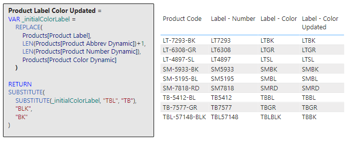
Product Label Color Updated =
VAR _initialColorLabel =    
    REPLACE(
        Products[Product Label],
        LEN(Products[Product Abbrev Dynamic])+1,
        LEN(Products[Product Number Dynamic]),
        Products[Product Color Dynamic]
    )

RETURN
SUBSTITUTE(
    SUBSTITUTE(_initialColorLabel, "TBL", "TB"),
    "BLK",
    "BK"
)

Here we start by defining the variable _initialColorLabel using the same expression as the previous example. Then we refine this with a double substitution! The inner SUBSTITUTE (SUBSTITUTE(_initialColorLabel, "TBL", "TB")) takes the initial label as the main text string and searches for TBL and replaces it with TB. The result of this (i.e. TBBLK) is then used as the initial text string for the outer SUBSTITUTE, which searches this string for BLK and replaces it with BK. This produces the new label that is consistent for all products.

Now we are starting to see the true power of DAX Text Functions, this expression does so much more than just a singular adjustment: it first reshapes the product label and then it goes even further to make sure the abbreviation and color codes that make up the label are consistent and concise. It is an illustration of how DAX can incrementally build and refine results for more accurate and streamlined outputs.

Although, these examples are helpful, it may be best to perform these transformations upstream when creating the dynamic extractions. For example the Product Abbrev Dynamic column we created early:

Product Abbrev Dynamic = 
LEFT(
  Products[Product Code], 
  FIND("-", Products[Product Code]) - 1
)

Could be updated to :

Product Abbrev Dynamic =
SUBSTITUTE (
    LEFT (
        Products[Product Code],
        FIND ( "-", Products[Product Code] ) - 1
    ),
    "TBL",
    "TB"
)

This would ensure consistency where ever the product code is used within the report.

As we continue our journey into the realm of DAX, remember that the right tool hinges on your specific needs. While CONCATENATE and COMBINEVALUES both join text strings, their nuanced differences could significantly influence the effectiveness of your data analysis and the presentation of your data. Choose wisely!


LEN & FORMAT — The Essentials

In the realm of DAX Text Functions, while both LEN and FORMAT serve distinct purposes, they play crucial roles in refining and presenting textual data. Throughout this deep dive into DAX Text Functions, you may have noticed these functions quietly powering several of our previous examples, working diligently behind the scenes.

For instance, in our Product Color Dynamic calculated column LEN was instrumental in determining the appropriate number of characters for the RIGHT function to extract. Similarly, our Yearly Page Title measure makes use of FORMAT, to ensure an aesthetic presentation of the YTD Sales value.

These instances highlight the versatility of LEN and FORMAT, illustrating how they can be combined with other DAX functions to achieve intricate data manipulations and presentation. Let’s take a look at the details of these two essential functions.

LEN Function: provides a straightforward way to understand the length of a text string and the syntax couldn’t be more simple.

LEN(text)

The text string you wish to know the length of is represented by “, just pass this to LEN to determine how many characters make up the string. The text string of interest could also be a column reference.

For more details see:

Learn more about: LEN

Now that you are more familiar with the LEN function revisit the previous examples to see it in action.

Product Color Dynamic =
VAR _firstHyphenPosition =
    FIND (
        "-",
        Products[Product Code]
    )
VAR _lastHyphenPosition =
    SEARCH (
        "-",
        Products[Product Code],
        _firstHyphenPosition + 1
    )
RETURN
    RIGHT (
        Products[Product Code],
        LEN ( Products[Product Code] ) - _lastHyphenPosition
    )
Product Label Color =
REPLACE (
    Products[Product Label],
    LEN ( Products[Product Abbrev Dynamic] ) + 1,
    LEN ( Products[Product Number Dynamic] ),
    Products[Product Color Dynamic]
)

FORMAT Function: reshapes how data is visually represented, with this function you can transition the format of data types like dates, numbers, or durations into standardized, localized, or customized textual formats. The syntax is as follows:

FORMAT(value, format_string[, locale_name])

Here, value represents the data value or expression that evaluates to a single value you intend to format and could be a number, date, or duration. The format string, format_string, is the formatting template and determines how the value will be presented. For example a format string of 'MMMM dd, yyyy' would present a value of 2023-05-12 as May 12, 2023. The locale_name is optional and allows you to specify a locale, different regions or countries may have varying conventions for presenting numbers, dates, or durations. Examples include en-US, fi-FI, or it-IT.

For more details see:

Learn more about: FORMAT

Now that you know the details of FORMAT see it put to work by revisiting the Yearly Page Title measure.

Yearly Page Title =
COMBINEVALUES (
    " ",
    YEAR (TODAY ()),
    "- Year to date sales:",
    FORMAT ([YTD Sales TOTALYTD], "Currency")
)

In this example, you see that the format_string uses a value of Currency to format the YTD sales. This is an example of a predefined numeric format. For more details on predefined numeric formats, custom numeric formats, custom numeric format characters, predefined date/time formats, and custom date/time formats visit the documentation here:


Beyond Strings: The Culmination of DAX Text Wisdom

Words share our world. And in the realm of data, they offer valuable insights. With DAX Text Functions, you have the power to manipulate, transform, and uncover these insights.

We have explored just a subset of DAX Text Functions during our journey here. There is still more to be uncovered so don’t stop learning here. Keep expanding and perfecting your DAX textual skills by exploring other text functions here:

Learn more about: Text functions

And, remember, anyone who has never made a mistake has never tried anything new. So, don’t be afraid of making mistakes; practice makes perfect. Continuously experiment and explore new DAX functions, and challenge yourself with real-world data scenarios.


Thank you for reading! Stay curious, and until next time, happy learning.

And, remember, as Albert Einstein once said, “Anyone who has never made a mistake has never tried anything new.” So, don’t be afraid of making mistakes, practice makes perfect. Continuously experiment and explore new DAX functions, and challenge yourself with real-world data scenarios.

If this sparked your curiosity, keep that spark alive and check back frequently. Better yet, be sure not to miss a post by subscribing! With each new post comes an opportunity to learn something new.

Time Travel in Power BI: Mastering Time Intelligence Functions


The Tools to Time Travel: An Introduction

In Power BI, time intelligence functions are your handy time machines. They enable you to extract useful insights from your data by manipulating time periods. These functions range from calculating sales year-to-date (YTD) to comparing data from previous years. If you want to unlock the true potential of your Power BI reports, you need to harness the might of Time Intelligence functions. In this post, we will unpack six time intelligence functions: DATESYTD, TOTALYTD, SAMEPERIODLASTYEAR, DATEADD, DATESINPERIOD, and DATESBETWEEN.

For those of you eager to start experimenting and diving deeper there is a Power BI report loaded with the sample data used in this post ready for you. So don’t just read, dive in and get hands-on with DAX Functions in Power BI. Check out it here:


The Twin Siblings: DATESYTD and TOTALYTD

First stop on our journey, the twin siblings, DATESYTD and TOTALYTD.

DATESYTD is the Einstein of the Power BI world, it uses the concept of relative time to help us compute values from the start of the year to the last date in the data. The syntax is as simple as the concept:

DATESYTD(dates[, year_end_dates])

Here, dates is a column containing dates, and year_end_date is an optional parameter to specify the year-end date, with a default value of December 31st.

On the other hand, TOTALYTD takes it up a notch. It summarizes data for the same period in a given year. The syntax of this function is:

TOTALYTD(expression, dates[, filter])

In this syntax, expression is what you want to calculate, dates is a column containing dates, and filter is a filter to restrict the calculation over time. TOTALYTD is DATESYTD, but with additional calculation power.

Here are example DAX formulas to calculate the total sales amount from the start of the year till the current date.

YTD Sales DATESYTD =
CALCULATE(
    SUM(Sales[Amount]),
    DATESYTD(Dates[Date])
)

And here is how you can calculate the same using TOTALYTD

YTD Sales TOTALYTD =
TOTALYTD(
  SUM(Sales[Amount]), 
  Dates[Date]
)

While both functions return the same result in this case, the key difference lies in their flexibility. DATESYTD just provides a set of dates, but TOTALYTD goes a step further to calculate an expression over those dates. Notice YTD Sales DATESYTD uses DATESYTD in combination with CALCULATE in order to achieve the same outcome as YTD Sales TOTALYTD.

For more information on these two head over to the Microsoft documentation for DATESYTD and TOTALYTD.

Learn more about: DATESYTD

Learn more about: TOTALYTD


The Cousins: SAMEPERIODLASTYEAR and DATEADD

Next up the cousins, SAMEPERIODLASTYEAR and DATEADD. SAMEPERIODLASTYEAR is the function that does exactly as the name suggests and always knows what happened “this time last year”. This is perfect for spotting trends, analyzing seasonality, or measuring growth. The syntax couldn’t be more straightforward:

SAMEPERIODLASTYEAR(dates)

Here, dates is a column that contains dates. Think of this function as equivalent to you Facebook memories, reminding you of what happened exactly one year ago.

DATEADD is the flexible function that allows you to go back (or forward) any number of intervals you choose. This handy function’s syntax is:

DATEADD(dates, number_of_intervals, interval)

Here, dates is your date column, number_of_intervals is the number of intervals to move (can be negative for moving backwards), interval and is the interval to use (DAY, MONTH, QUARTER, or YEAR). This function lets you journey backward or forward in time with ease!

The example for this duo calculates the total sales for the same period in the previous year. The DAX formula for this example is:

Sales LY SAMEPERIODLASTYEAR =
CALCULATE(
    SUM(Sales[Amount]),
    SAMEPERIODLASTYEAR(Dates[Date])
)

Similarly, using DATEADD, you can achieve the same result by subtracting one year from the current date:

Sales LY DATEADD =
CALCULATE(
    SUM(Sales[Amount]),
    DATEADD(Dates[Date], -1, YEAR)
)

While both of these functions seem to do the same job, the difference again lies in their flexibility. SAMEPERIODLASTYEAR only takes you back one year, while DATEADD give you the liberty to move as far back or forward as you want, making it a more flexible option overall.

Visit the Microsoft documentation for SAMEPERIODLASTYEAR and DATEADD for a deeper dive.

Learn more about: SAMEPERIODLASTYEAR

Learn more about: DATEADD


The Mysterious Pair: DATESINPERIOD and DATESBETWEEN

Last but not least, let’s explore the mysterious pair DATESINPERIOD and DATESBETWEEN. DATESINPERIOD has your back if you need to calculate data for a specific period. It returns a table that contains a column of dates that starts from a specific date, extends by a specified interval, and stops at the end of the last interval.

Its syntax is:

DATESINPERIOD(dates, start_date, number_of_intervals, interval)

Here, dates is a column containing dates, start_date is the start date for the calculation, number_of_intervals is the number of intervals to include, and is the interval to use (DAY, MONTH, QUARTER, or YEAR).

DATESBETWEEN, however, is the function you’d use to fetch data between two specific dates. It returns a table that contains a column of all dates between two specified dates. The syntax is as simple as:

DATESBETWEEN(dates, start_date, end_date)

Here, dates is a column that contains dates, start_date is the start date for the calculation, and end_date is the end date for the calculation. It’s like ordering a specific range of books from a library catalog. You get exactly what you want, nothing more, nothing less!

Let’s look at a practical example of these functions. Say you want to calculate the 3-month rolling average sales, both these functions can help solve this in their own way.

Using DATAINPERIOD the DAX formula is:

Sales 3 Month Rolling Average DATESINPERIOD =
CALCULATE(
    AVERAGE(Sales[Amount]),
    DATESINPERIOD(Dates[Date], LASTDATE(Dates[Date]), -3, MONTH)
)

This formula calculates the average sales for the previous three months from the last date in the data. The same calculation with DATESBETWEEN would like like:

Sales 3 Month Rolling Average DATESBETWEEN =
CALCULATE(
    AVERAGE(Sales[Amount]),
    DATESBETWEEN(
        Dates[Date],
        EDATE(LASTDATE(Dates[Date]), -3),
        LASTDATE(Dates[Date])
    )
)

This formula also returns the average sales for the previous three months from the last date in the data. The key difference is that with DATESBETWEEN, you explicitly specify the start and end dates, providing a high degree of precision when needed.

You can learn more about these functions at the Microsoft documentation for DATESINPERIOD and DATESBEETWEEN.

Learn more about: DATESINPERIOD

Learn more about: DATESBETWEEN


Stepping Out of the Time Capsule

Power BI’s Time Intelligence functions are akin to a time-traveling journey. They empower you to traverse through your data — past, present, and future. Whether you’re revisiting the past year with SAMEPERIODLASTYEAR, leaping through your data with DATEADD, or meticulously exploring specific date ranges with DATESBETWEEN, the power is all yours. So fasten your seat belts, prepare your time capsules, and commandeer your data journey. Happy data crunching!

And remember, as Albert Einstein once said, “Anyone who has never made a mistake has never tried anything new.” So, don’t be afraid of making mistakes; practice makes perfect.

Continuously experiment with Time Intelligence functions, explore new DAX functions, and challenge yourself with real-world data scenarios.


Thank you for reading! Stay curious, and until next time, happy learning.

And, remember, as Albert Einstein once said, “Anyone who has never made a mistake has never tried anything new.” So, don’t be afraid of making mistakes, practice makes perfect. Continuously experiment and explore new DAX functions, and challenge yourself with real-world data scenarios.

If this sparked your curiosity, keep that spark alive and check back frequently. Better yet, be sure not to miss a post by subscribing! With each new post comes an opportunity to learn something new.

Power BI Context Transition: Navigating the Transition between Row and Filter Contexts

Series Review

One of the early stages of creating any Power BI report is the development of the data model. The data model will consist of data tables, relationships, and calculations. There are two types of calculations: calculated columns, and measures.

Check out Power BI Row Context: Understanding the Power of Context in Calculations for key differences between calculated columns and measures.

Row Context — What it is, When is it available, and its Implications

One of the most powerful elements of Power BI is that all measure calculations are done in context. The evaluation context limits the values in the current scope when evaluating an expression. The filter context and/or the row context make up the evaluation context.

Power BI Row Context: Understanding the Power of Context in Calculations of this series explores the row context in depth.

While Power BI Iterators: Unleashing the Power of Iteration in Power BI Calculations explores iterator functions, which are functions that create row context.

Iterator Functions — What they are and What they do

And finally, Power BI Filter Context: Unraveling the Impact of Filters on Calculations explores the concept of the filter context.

Filter Context – How to create it and its impact on measures

When evaluating expressions, the row context can be transitioned into a filter context within Power BI. This transition can help create more complex measures. Row context, filter context, and context transition can be confusing when starting with DAX so visit references and documentation often.

This post is the fourth of a Power BI Fundamental series with a focus on the context transition. The example file used in this post is can be found on GitHub at the link below.

Power BI key fundamentals example files


Understanding Context Transition

The row context by itself does not filter data. Row context iterates through a table row-by-row. Context transition is when the row context transitions into the filter context. Context transition occurs with the CALCULATE() function and when the expression of an iterator function is a DAX measure.

The concept of context transition can be a bit abstract so it can be easiest to learn through examples. To explore, we will create a new calculated column in the Products table. The new ProductsSales calculates the total sales for each product and we define it as:

ProductSales = 
SUM(SalesOrderDetail[SalesAmount])

After evaluating ProductSales we see it repeats the same $109.85M sales value for each row. This value is the total sales amount for the entire dataset. This is not what we want ProductSales to calculate, so what happened?

ProductSales calculates the total sales of the entire data rather than the filtered per-product value because row context is not a filter. For example, the row context includes the ProductID value but this identifier is not a filter on the data during evaluation. And because the row context is not a filter DAX does not distinguish between different rows (i.e products) when evaluating ProductSales.

For example, looking at the table above while evaluating the measure DAX does not distinguish the Adjustable Race row from the LL Crankarm row. Since all rows are viewed as the same the total sales value is repeated for each row.

You may have guessed it but, the example above calculates the wrong value because it does not contain a context transition. The row context does not shift to the filter context causing the error in the calculated value. This simple example highlights why context transition is important and when it’s needed. To correct this we must force the context transition. This will convert the row values into a filter and calculate the sales for each product. There are various ways to do this, and below are two options.

Option #1: The CALCULATE() Function

We can force context transition by wrapping ProductSales with the CALCULATE() function. To demonstrate we create a new ProductSales_calculate column. ProductSales_calculate is defined as:

ProductSales_calculate = 
CALCULATE(
   SUM(SalesOrderDetail[SalesAmount])
)

This new calculated column shows the correct sales value for each product. We view the product type BK and can see now each row in the ProductSales_calculate column is different for each row.

Option #2: Using Measures

Within the data model, we have already created a measure SalesAmount2.

We defined SalesAmount2 as:

SalesAmount2 = 
SUMX(
   SalesOrderDetail, 
   SalesOrderDetail[OrderQty] * SalesOrderDetail[UnitPrice] * (1 - 
   SalesOrderDetail[UnitPriceDiscount])
)

We can see by the expression SalesAmount2 uses the iterator function SUMX(). This measure calculates the sales amount row-by-row in the SalesOrderDetail table. As mentioned before context transition occurs within iterator functions. So rather than using CALCULATE() and SUM() we create another calculated column that references this measure.

ProductSales_measure = SalesAmount2

We add the new column to the table visual and can see that it has the same value as ProductSales_calculate. This shows that a measure defined with an iterator also forces context transition.

An important note about this new column is that the ProductsSales_measure works as expected when referencing the measure. However, it will not work if we define this column as the same expression that defines SalesAmount2.

We can see below if we update ProductSales_measure to:

SUMX(
   SalesOrderDetail, 
  SalesOrderDetail[OrderQty] * SalesOrderDetail[UnitPrice] * (1 - 
  SalesOrderDetail[UnitPriceDiscount])
)

The same expression used when defining SalesAmount2, will result in wrong values.

After updating ProductSales_measure we can see it returns the total sales values and not the sales per product. With this updated definition DAX is no longer able to apply the context transition. We can correct this by wrapping the expression with CALCULATE().


Maximum Daily Sales by Month Example

A question of interest is what is the maximum daily sales amount for each month in the dataset. In other words we would like to determine for each month what day of the month had the highest sales and what was the total daily sales value. We start by creating a new MaxDailySales measure and add it to the Max Daily Sales by Month and Year table visual.

We define MaxDailySales as:

MaxDailySales = 
MAXX(SalesOrderDetail, [SalesAmount2])

After adding the measure to the table we can see the sales amount value for each month. For example, the table currently shows that the maximum daily sales for November 2016 is $21,202.79. This value may appear reasonable but when examined closely we can determine it is incorrect. Currently, MaxDailySales is returning the maximum sale for each month and is not accounting for multiple sales within each day. We can see this by creating a new visual with the Date, MaxSales, and SalesOrderDetailID fields.

This table shows that the MaxDailySales for November 2016 is the same value as a single sale that occurred on November 17th. Yet, there are multiple sales on this day and every other day. The desired outcome is to calculate the total sales for each day and then determined the highest daily total value for each month.

This error occurs because context transition is not being applied correctly. It is important to note that context transition is occurring while evaluating MaxDailySales because it is a measure. However, the context transition is not being applied on the correct aggregation level. The context transition is occurring on the SalesOrderDetail level, meaning for each row of this table. To correct this measure we will have to force the context transition on the correct, daily, aggregation level. We update the MaxDailySales expression using the VALUES() function.

We define MaxDailySales_Corrected as:

MaxDailySales_Corrected = 
MAXX(
   VALUES(DateTable[Date]), 
   [SalesAmount2]
)

We change the table passed to MAXX() from SalesOrderDetail to VALUES(DateTable[Date]). Using VALUES(DateTable[Date]) aggregates all the dates that are the same day shifting the context transition to the correct aggregation level. The VALUES() function in the expression provides a unique list of dates. For each day in the unique list, the SalesAmount2 measure gets evaluated and returns the maximum daily total value. We then add the new measure to the table visual and now it shows the correct maximum daily sales for each month.

The above example shows context transition at two different aggregation levels. They also highlight that the context transition can be shifted to return the specific value that is required. As well as showing why it is important to take into consideration the aggregation level when developing measures like MaxDailySales.


Context Transition Pit Falls

Context transition is when row values transition into or replace the filter context. When context transition occurs it can sometimes lead to unexpected and incorrect values. An important part of context transition to understand is that it transitions the entire row into the filter. So what occurs when a row is not unique? Let’s explore this with the following example.

We add a new SimplifiedSales table to the data model.

Then we add a TotalSales measure. TotalSales is defined as:

TotalSales = 
SUMX(
   SimplifiedSales, 
   SimplifiedSales[OrderQty] * SimplifiedSales[UnitPrice] * (1 - 
   SimplifiedSales[UnitPriceDiscount])
)

Viewing the two tables above, we can confirm that the TotalSales values are correctly aggregating the sales data. Now we add another measure to the table which references the measure TotalSales. Referencing this measure will force context transition due to the implicit CALCULATE() added to measures. See above for details.

We define TotalSales_ConextT as:

TotalSales_ContextT = 
SUMX(SimplifiedSales, [TotalSales])

In the new column we can see that the values for Road-350-W Yellow, 48 and Touring-3000 Blue, 44 have not changed and are correct. However, Mountain-500 Silver, 52 did update, and TotalSales_ContextT column shows an incorrect value. So what happened?

The issue is the context transition. Viewing the SimplifiedSales table we can see that Mountain-500 Silver, 52 appears twice in the table. With both records having identical values for each field. Remember, context transition utilizes the entire row. Meaning the table gets filtered on Mountain-500 Silver, 52/ 1/$450.00. Because of this, the result gets summed up in the TotalSales measure returning a value of $900.00. This value is then evaluated twice, once for each identical row.

This behavior is not seen for the Road-350-W, 48 records because they are unique. One row has a UnitPriceDiscount of 0.0% and the other has a value of 5.0%. This difference makes each row unique when context transition is applied.

Knowing what context transition is and when it occurs is important to identifying when this issue may occur. When context transition is applied it is important to check the table and verify calculations to ensure it is applied correctly.


Thank you for reading! Stay curious, and until next time, happy learning.

And, remember, as Albert Einstein once said, “Anyone who has never made a mistake has never tried anything new.” So, don’t be afraid of making mistakes, practice makes perfect. Continuously experiment and explore new DAX functions, and challenge yourself with real-world data scenarios.

If this sparked your curiosity, keep that spark alive and check back frequently. Better yet, be sure not to miss a post by subscribing! With each new post comes an opportunity to learn something new.

Power BI Filter Context: Unraveling the Impact of Filters on Calculations

Series Review

One of the early stages of creating any Power BI report is the development of the data model. The data model will consist of data tables, relationships, and calculations. There are two types of calculations: calculated columns, and measures.

Check out Power BI Row Context: Understanding the Power of Context in Calculations for key differences between calculated columns and measures.

Row Context — What it is, When is it available, and its Implications

All expressions, either from a calculated column or a measure, get evaluated within the evaluation context. The evaluation context limits the values in the current scope when evaluating an expression. The filter context and/or the row context make up the evaluation context.

Power BI Row Context: Understanding the Power of Context in Calculations explores the row context in depth. While Power BI Iterators: Unleashing the Power of Iteration in Power BI Calculations explores iterator functions, which are functions that create row context.

Iterator Functions — What they are and What they do

This article is the third of a Power BI Fundamental series with a focus on the filter context. The example file used in this post is located here – GitHub.


Introduction to Filter Context

Filter context refers to the filters applied before evaluating an expression. This filter context limits the set of rows of a table available to the calculation. There are two types of filters to consider, the first is implicit filters or filters applied by the user via the report canvas. The second type is explicit filters which use functions such as CALCULATE() or CALCULATETABLE().

The applied filter context can contain one or many filters. When there are many filters the filter context will be the intersection of all the filters. When the filter context is empty all the data is used during the evaluation.

Filter context propagates through the data model relationships. When defining each model relationship the cross-filter direction is set. This setting determines the direction(s) the filters will propagate. The available cross-filter options depend on the cardinality type of the relationship. See available documentation for more information on Cross-filter Direction and Enabling Bidirectional Cross-filtering.

It is important to be familiar with certain DAX functions which can modify the filter context. Some examples used in the post include CALCULATE()ALL(), and FILTER().


The CALCULATE Function

The CALCULATE() function can add filters to a measure expression, ignore filters applied to a table, or overwrite filters applied from within the report visuals. The CALCULATE() function is a powerful and important tool when updating or modifying the filter context.

The syntax of CALCULATE() is:

CALCULATE(<expression>, <filter1>, <filter2>, ...)

Use the CALCULATE() function when modifying the filter context of an expression that returns a scalar value. Use CALCULATETABLE() when modifying the filter context of an expression that returns a table.


Exploring Filter Context

The table below is a visualization of the total sales amount for each product color.

The table visual creates filter context, as seen by the total sales amount for each color or row. Evaluating SalesAmount2 occurs by first filtering the SalesOrderDetail table by the color, and then evaluating the measure with the filtered table. This is then repeated for each product color in the SalesOrderDetail table.

The above example only contained the single product color filter. However, as mentioned previously, the filter context can contain multiple filters. The example table below adds the ProductType to the table. The addition of this field breaks down the total sales first by color and then by product type. For each row, the underlying SalesOrderDetail table is first filtered by color and product type before evaluating the SalesAmount2 measure. In these examples, it is the table visual that is creating the filter context.


Create Filter Context with Slicers

Another way to create filter context is through the use of slicer visuals. For this example, a slicer of the ProductType is created.

When no value is selected in the slicer the filter context from the slicer visual is null. Meaning at first the card visual shows the SalesAmount2 value evaluated for all data. Additionally, when no value is selected in the slicer the only filter context is ProductColor from the table visual.

Following the selection of BK in the product type slicer, the values in both the table and the card visual are updated. The card visual now has one filter context which is the product type BK. This is evaluated by creating a filtered table and SalesAmount2 is evaluated for this filtered table.

The SalesAmount2 measure is defined by:

SalesAmount2 =
SUMX (
    SalesOrderDetail,
    SalesOrderDetail[OrderQty] * SalesOrderDetail[UnitPrice] * 
    ( 1 - SalesOrderDetail[UnitPriceDiscount] )
)

After selecting an option from the slicer the measure is re-evaluated. The re-evaluation occurs to account for the newly created filter context. The filter context creates a subset of the SalesOrderDetail table that matches the slicer selection. Then the row context evaluates the expression row-by-row for the filtered table and is summed. SUMX() is an example of an iterator function, see Power BI Iterators: Unleashing the Power of Iteration in Power BI Calculations for more details. The updated value is then displayed on the card visual.

Iterator Functions — What they are and What they do

The table visual works in a similar fashion but, there are two filters applied. The table visual has an initial filter context of the product color. After the selection of BK, the table gets updated to visualize the intersection of the product color filter and the product type filter.

Following a selection in the slicer visual, if a row in the table visual is selected this will also apply a filter. The filter context is the intersection of the table selection filters and the slicer. The updated filter context gets applied to all other visuals (e.g. the card visual).


Create Filter Context with CALCULATE

Previous examples created the filter context using implicit filters. Generally, the user creates this type of filter through the user interface. Another way to create filter context is by using explicit filters. Explicit filters get created through the use of functions such as CALCULATE(). For this example, rather than having to select BK in the slicer to view total bike sales, we will use CALCULATE(). We will create a new measure that will force the filter context. We can do this because CALCULATE() allows us to set the filter context for an expression.

We define the BikeSales measure as:

BikeSales =
CALCULATE ( 
   SalesOrderDetail[SalesAmount2], 
   Products[ProductType] = "BK" 
)
  • Expression: SalesOrderDetails[SalesAmount2]
  • Filter: Products[ProductType]="BK"

BikeSales is then added to the table visual alongside SalesAmount2. When the BK product type is the slicer selection the two table columns are equal. Both measures have the same filter context created by product color and product type. Removing the implicit product type filter by unselecting a product type updates the filter context. The SalesAmount2 expression is re-evaluated with the updated filter context. Since the filter context created by the slicer is now null the SalesAmount2 value calculates using all the data. The BikeSales values do not change. This is because of the explicit filter used by the CALCULATE() function when we defined the measure. The BikeSales measure still has the filter Products[ProductType]="BK" applied regardless of the product type slicer.

The CALCULATE() function only creates filter context and does not create row context. So an important question to ask is why or how the BikeSales measure works. The CALCULATE() function references a specific column value, Products[ProductType]="BK". Yet, the CALCULATE() function does not have row context. So how does Power BI know which row it is working with? The answer is that the CALCULATE() function applies the FILTER() function. And the FILTER function creates the row context required to evaluate the measure.

Within the CALCULATE() function the Products[ProductType]="BK filter is shorten syntax. The filter argument passed to CALCULATE() is equivalent to FILTER(ALL(Products[ProductType]), Products[ProductType]="BK")). The ALL() function removes any external filters on the ProductType column and is another example of a function that can modify the filter context.

Keep External filters with CALCULATE

The CALCULATE() function evaluates the filter context both outside of and within the function. The filter context outside of the function can come from user interaction with visuals. The filter context within the function is the filter expression(s).

To explore this we create a table with the Product Type, SalesAmount2, and SalesBike.

The SalesAmount2 column shows the total sales amount, if any, as expected. While the BikeSales column shows the same repeated value for all rows and is incorrect. Looking at the Product Type BK row we can see this row is correct. This table demonstrates that CALCULATE()overwrites external filters.

For example, the BB product type row filters SalesOrderDetail before evaluating SalesAmount2. This returns the correct total sales for the BB product type. When evaluating BikeSales this external product type filter gets overwritten. The measure calculates the sales amount value for the BK product type due to the explicit filter and returns this value for all rows.

Using the KEEPFILTERS() function within CALCULATE() will force CALCULATE() to keep both external and internal filters.

To do this we update BikeSales to:

BikeSales = 
CALCULATE(
   SalesOrderDetail[SalesAmount2], 
   KEEPFILTERS(Products[ProductType]="BK")
)

After updating the measure definition the resulting table is shown below.

Keeping the external filters is shown by the empty values for all rows except BK. For example, we look again at the BB product type row. When evaluating BikeSales Power BI keeps the external filter Products[ProductType]="BB" and the internal filter Products[ProductType]="BK". When applying more than one filter the filter context is the intersection of the two. The intersection of the two applied filters for the BB row is empty. A product cannot be both of type BB and BK.


More CALCULATE Examples

The CALCULATE() function plays an integral part in the filter context. Below are more examples to show key concepts and show that CALCULATE() is an important part of the filter context.

Creating a measure of High Quantity Sales

For the first example, we will be creating a sales measure showing the total sales amount for high-quantity orders. Creating this measure requires first filtering the SalesOrderDetail table based on the OrderQty. Then evaluating the SalesAmount2 measure with this filtered table.

We define HighQtySales as:

HighQtySales = 
CALCULATE(
   [SalesAmount2], 
   SalesOrderDetail[OrderQty]>25
)

We then visualize this measure on a card visual and see that 96.30K of our total 109.85M sales come from a high-quantity order. This again demonstrates the filter arguments passed to CALCULATE() are shorthand syntax. The filter arguments within CALCULATE() use the FILTER() function to create the row context required. In this example SalesOrderDetail[OrderQty]>25 is equivalent to FILTER(ALL(SalesOrderDetail),SalesOrderDetail[OrderQty] > 25).

The FILTER() function is an example of an iterator function and creates the row context. The row context allows for row-by-row evaluation of the OrderQty. Meaning it evaluates SalesOrderDetail[OrderQty] > 25 for each row of the SalesOrderDetail table. FILTER() then returns a virtual tale that is a subset of the original and contains only orders with a quantity greater than 25.

Percentage of Sales by Product Color

For the second example, we will create a measure to show the percentage of total sales for each product color. To create this we will start with a new AllSales measure. AllSales uses the CALCULATE() function to remove any filters and evaluates SalesAmount2.

We define AllSales as:

AllSales = 
CALCULATE(
   [SalesAmount2], 
   ALL(Products[Color])
)

AllSales is then added to the table visual Percentage of Sales by Color. Once added the AllSales column shows 190.85M total sales value for each color. This is consistent with the SalesAmount2 card visual. Repeating this value for each color is also expected because of the filter expression ALL(Products[Color]).

ALL(Products[Color]) creates a new filter context and gets evaluated with any other filters from the visuals. In this example, CALCULATE() overwrites any external filters on Products[Color]. This is why once added to the table visual AllSales displays the total sales value repeated for each row.

The ALL() function removes any filter limiting the color column that may exist while evaluating AllSales. It is best practice to define a measure as specific as possible. Notice, in this example ALL() applies to Product[Color], rather than the entire Product table. If other filters exist on other columns from the visuals these filters will still impact the evaluation. For example, selecting a product type from the slicer will adjust all values.

Following the selection, SalesAmount2 represents the total BK sales for each color. While the AllSales measure now represents the total sales for all BK product types. This occurs because when there are multiple filters the result is the intersection of all the filters.

In this case, All(Product[Color]) removes the filter on the color column. The slicer visual creates an external filter context of only BK product types. During the evaluation, the intersection of these two creates the evaluation context.

We can also remove the external filter context created by the product type slicer. To do this, we update the AllSales measure to include Products[ProductType] as an additional filter argument.

We update the filter expression of the CALCULATE() function to:

AllSales = 
CALCULATE(
   [SalesAmount2], 
   ALL(Products[Color], 
   Products[ProductType]
)

After updating the measure the AllSales column of the table visual updates to the total sales value. The column now displays the expected 109.85M value and is no longer impacted by the filter context created by the slicer visual.

Another option to remove the filter context within CALCULATE() is to use the REMOVEFILTER() function.

AllSales = 
CALCULATE(
   SalesOrderDetail[SalesAmount2], 
   REMOVEFILTERS(
      Products[Color], 
      Products[ProductType]
   )
)

We created AllSales as an initial step of the broader goal to calculate the percentage of total sales. To calculate the percentage we will update the AllSales expression. We can do this by saving the AllSales expression as a variable within the measure. We will also create another variable to store the SalesAmount2 value, which will be the total sales for each product color. Lastly, we will update the measure name to PercentageSales which will RETURN the division of the two sales variables.

PercentageSales =
VAR Sales = SalesOrderDetail[SalesAmount2]
VAR AllSales = 
CALCULATE(
   SalesOrderDetail[SalesAmount2], 
   REMOVEFILTERS(
      Products[Color],
      Products[ProductType]
   )
)

RETURN
DIVIDE(Sales, AllSales)

Thank you for reading! Stay curious, and until next time, happy learning.

And, remember, as Albert Einstein once said, “Anyone who has never made a mistake has never tried anything new.” So, don’t be afraid of making mistakes, practice makes perfect. Continuously experiment and explore new DAX functions, and challenge yourself with real-world data scenarios.

If this sparked your curiosity, keep that spark alive and check back frequently. Better yet, be sure not to miss a post by subscribing! With each new post comes an opportunity to learn something new.

Power BI Iterators: Unleashing the Power of Iteration in Power BI Calculations

Overview

In order to facilitate analysis and visualization in Power BI a data model must first be created. The data model consists of individual data tables, relationships, and calculations. Calculations come in the form of either calculated columns or measures.

Check out this post to explore the key differences between calculated columns and measures.

Row Context — What it is, When is it available, and its Implications

The evaluation context limits the values in the current scope when Power BI evaluates a DAX expression. There are two types of evaluation context, filter and row, that can be active during the evaluation of a DAX expression.

This post is the second of a Power BI Fundamental series with a focus on iterator functions. The example file used in this post is located found on GitHub at the link below.

Power BI key fundamentals example files


Introduction

This post will build upon the Power BI file created in Part 1 of the series titled row_context_example. The example file for this post is iterator_functions, and both can be found on GitHub at the link above.

As noted at the end of Power BI Row Context: Understanding the Power of Context in Calculations, creating a measure by default was unable to reference the row values of a column. When creating a measure a column can be referenced and passed to a standard aggregation function. The standard aggregation function will return only a single aggregated value. This is not the row-by-row functionality that will be required to replace a calculated column, such as SalesAmount found in the SalesOrderDetail table.

Creating the desired measure will require an iterator function to create row context.

Understanding Iterators

An iterator moves row-by-row or iterates through an object. The object can be a data model table or a virtual/temporary table. Data model tables are tables loaded into or linked to within Power BI. A table generated from within a measure that persists only for a temporary period of time is a virtual table.

An iterator function can return a single value (e.g. number, text, date) or a virtual table. An iterator generally has two arguments:

  • The object (i.e. table) to iterate through
  • The expression evaluated for each row of the object

It can be helpful to think of the expression as a temporary column of the object. Evaluation of the expression occurs row-by-row creating a column of calculated results. The column of results only persists during the evaluation and is not loaded to the data model. The purpose of the temporary column is to calculate the final returned value of the iterator.

Examples of iterator functions include SUMXMINXMAXXAVERAGEX, and RANKX. The ending X is only a common identifier, FILTER is an example of an iterator function that does not end with a X.

Example iterator function:

SUMX(
   SalesOrderDetail, 
   SalesOrderDetail[OrderQty] * SalesOrderDetail[UnitPrice] * (1 - SalesOrderDetail[UnitPriceDiscount])
)
  • Table: SalesOrderDetail – the object iterated over
  • Expression: SalesOrderDetail[OrderQty] * SalesOrderDetail[UnitPrice] * (1 - SalesOrderDetail[UnitPriceDiscount]) – the expression evaluated for each row.

Once implementing the iterator SUMX and specifying the table as SalesOrderDetails the columns of the table will be recognized and able to be referenced like when a calculated column was created. The new measure SalesAmount2 created using an iterator will replace the calculated column SalesAmount. Comparing the default aggregation of the SalesAmount column (i.e. Sum of SalesAmount) and the new measure SalesAmount2 it can been see the values are equal.


Iterator Functions that Generate Virtual Tables

There are iterator functions such as SUMX that return a scalar value and there are ones like FILTER that return virtual tables.

To further explore, first create a new table in the data model generated by the returned table of the FILTER function.

For this example, we use the FILTER function to create a new ProductBlue table. For the first argument of the FILTER function we pass in the Product table. Then we filter that table using a filter expression defined as Products[Color] = "blue".

ProductBlue = FILTER(Products, Products[Color] = "blue")

We then can visualize this new table and compare the row count to the count of ProductID by color of the original table. Comparing these two tables we see that ProductBlue is a subset of the Product table.

The generation of this table highlights the iterating functionality and the row context when evaluating the FILTER function. To create the ProductBlue table the FILTER iterator function must create row context. During the evaluation, the function must go within the Products table and for each row (i.e. row context) evaluate what the product color is. If the color is Blue the function returns True otherwise returns False. The resulting table then consists of only rows from the original table which evaluated to a value of True.

Creating the new ProductBlue table was for demonstrative purposes. The table returned by FILTER can be a virtual table used within a measure. In this case, the ProductBlue table would only persist while the measure is being evaluated. As an example, create a new ProductBlueMeasure measure using the COUNTROWS function. COUNTROWS takes a single argument, the table to count the row of. To do this we will pass the FILTER expression used to create the ProductBlue table to the COUNTROWS function. To further demonstrate that the ProductBlue table is unnecessary, we can create a similar ProductBlackMeasure by changing =”blue" to =”black". Viewing these measures shows the result is the same counts that were produced by the other methods used to obtain this count.


Combining Iterators

More complex measures can be created by combining or nesting iterators. For example, combining the product color and the sales data, such as evaluating the total sales for only blue products. This measure will first create a virtual table of the sales data for only blue products. Then iterate row-by-row through the virtual table and evaluate the sales amount. Finally, return the total sales amount.

The DAX expression will be:

SUMX(
   FILTER(
      SalesOrderDetail, 
      RELATED(Products[Color])="Blue"
   ), 
  SalesOrderDetail[OrderQty] * SalesOrderDetail[UnitPrice] * (1 - SalesOrderDetail[UnitPriceDiscount])
)

The virtual table mentioned above is generated by FILTER(SalesOrderDetail, RELATED(Products[Color])="Blue").
This is the first iterator function that is evaluated using the SalesOrderDetail table and the expression RELATED(Products[Color])="Blue".

RELATED() is a function that returns a related value from another table. This function can be used since the Product table is related to the SalesOrderDetail table with a key value of ProductID. The FILTER function then returns a subset of the SalesOrderDetail table containing only rows where the product is blue. This virtual table is then passed to SUMX.

Then the expression evaluated row-by-row is:

SalesOrderDetail[OrderQty] * SalesOrderDetail[UnitPrice] * (1 - SalesOrderDetail[UnitPriceDiscount])

Which returns the total sales amount for each row. Then this temporary column is summed by the SUMX function.

Viewing the two tables on the left, the totals sales for the Blue products for all methods is approximately 9.60M. Selecting the blue row in the top table filters the table below, to show sales by Product for only blue products. Viewing the totals for all three methods also shows a value of approximately 9.60M. Lastly, viewing the value card under Nested Iterator shows that the above created DAX expressions results in the same value of 9.60M.

Key concepts are highlighted in the above example

  • Both SUMX and FILTER create row context
  • The FILTER function returns a virtual table which is a subset of SalesOrderDetail
  • SUMX returns the sum of the row-by-row calculation of the sale amount
  • The table passed to SUMX is the table that is returned by the FILTER function, this table only persists during the evaluation of SUMX

The concept of evaluation context has been mentioned in this post as well as in the previous post – Power BI Row Context: Understanding the Power of Context in Calculations.

Row Context — What it is, When is it available, and its Implications

Evaluation context is the context in which a DAX formula evaluates a calculation. There are two types, Power BI Row Context: Understanding the Power of Context in Calculations explored the first type, row context. This post explored iterators or specific functions which create row context to perform multi-column calculations. Check out Part Three of this series which will explore the second type of evaluation context, the filter context.

Filter Context – How to create it and its impact on measures


Thank you for reading! Stay curious, and until next time, happy learning.

And, remember, as Albert Einstein once said, “Anyone who has never made a mistake has never tried anything new.” So, don’t be afraid of making mistakes, practice makes perfect. Continuously experiment and explore new DAX functions, and challenge yourself with real-world data scenarios.

If this sparked your curiosity, keep that spark alive and check back frequently. Better yet, be sure not to miss a post by subscribing! With each new post comes an opportunity to learn something new.