
Iterator Functions — What they are and What they do
Overview
In order to facilitate analysis and visualization in Power BI a data model must first be created. The data model consists of individual data tables, relationships, and calculations. Calculations come in the form of either calculated columns or measures.
Check out this post to explore the key differences between calculated columns and measures.

Power BI Row Context: Understanding the Power of Context in Calculations
Row Context — What it is, When is it available, and its Implications
The evaluation context limits the values in the current scope when Power BI evaluates a DAX expression. There are two types of evaluation context, filter and row, that can be active during the evaluation of a DAX expression.
This post is the second of a Power BI Fundamental series with a focus on iterator functions. The example file used in this post is located found on GitHub at the link below.

GitHub – Power BI Key Fundamentals
Power BI key fundamentals example files
Introduction
This post will build upon the Power BI file created in Part 1 of the series titled row_context_example. The example file for this post is iterator_functions, and both can be found on GitHub at the link above.
As noted at the end of Power BI Row Context: Understanding the Power of Context in Calculations, creating a measure by default was unable to reference the row values of a column. When creating a measure a column can be referenced and passed to a standard aggregation function. The standard aggregation function will return only a single aggregated value. This is not the row-by-row functionality that will be required to replace a calculated column, such as SalesAmount found in the SalesOrderDetail table.
Creating the desired measure will require an iterator function to create row context.
Understanding Iterators
An iterator moves row-by-row or iterates through an object. The object can be a data model table or a virtual/temporary table. Data model tables are tables loaded into or linked to within Power BI. A table generated from within a measure that persists only for a temporary period of time is a virtual table.
Since an iterator moves row-by-row it has row context, and row context always iterates
An iterator function can return a single value (e.g. number, text, date) or a virtual table. An iterator generally has two arguments:
- The object (i.e. table) to iterate through
- The expression evaluated for each row of the object
It can be helpful to think of the expression as a temporary column of the object. Evaluation of the expression occurs row-by-row creating a column of calculated results. The column of results only persists during the evaluation and is not loaded to the data model. The purpose of the temporary column is to calculate the final returned value of the iterator.
A common identifier of an iterator function is an X at the end of the function’s name
Examples of iterator functions include SUMX, MINX, MAXX, AVERAGEX, and RANKX. The ending X is only a common identifier, FILTER is an example of an iterator function that does not end with a X.
Example iterator function:
SUMX(
   SalesOrderDetail,
   SalesOrderDetail[OrderQty] * SalesOrderDetail[UnitPrice] * (1 - SalesOrderDetail[UnitPriceDiscount])
)
- Table:
SalesOrderDetail– the object iterated over - Expression:
SalesOrderDetail[OrderQty] * SalesOrderDetail[UnitPrice] * (1 - SalesOrderDetail[UnitPriceDiscount])– the expression evaluated for each row.
Once implementing the iterator SUMX and specifying the table as SalesOrderDetails the columns of the table will be recognized and able to be referenced like when a calculated column was created. The new measure SalesAmount2 created using an iterator will replace the calculated column SalesAmount. Comparing the default aggregation of the SalesAmount column (i.e. Sum of SalesAmount) and the new measure SalesAmount2 it can been see the values are equal.

Iterator Functions that Generate Virtual Tables
There are iterator functions such as SUMX that return a scalar value and there are ones like FILTER that return virtual tables.
To further explore, first create a new table in the data model generated by the returned table of the FILTER function.
For this example, we use the FILTER function to create a new ProductBlue table. For the first argument of the FILTER function we pass in the Product table. Then we filter that table using a filter expression defined as Products[Color] = "blue".
ProductBlue = FILTER(Products, Products[Color] = "blue")
We then can visualize this new table and compare the row count to the count of ProductID by color of the original table. Comparing these two tables we see that ProductBlue is a subset of the Product table.
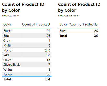
The generation of this table highlights the iterating functionality and the row context when evaluating the FILTER function. To create the ProductBlue table the FILTER iterator function must create row context. During the evaluation, the function must go within the Products table and for each row (i.e. row context) evaluate what the product color is. If the color is Blue the function returns True otherwise returns False. The resulting table then consists of only rows from the original table which evaluated to a value of True.
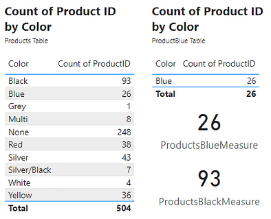
Creating the new ProductBlue table was for demonstrative purposes. The table returned by FILTER can be a virtual table used within a measure. In this case, the ProductBlue table would only persist while the measure is being evaluated. As an example, create a new ProductBlueMeasure measure using the COUNTROWS function. COUNTROWS takes a single argument, the table to count the row of. To do this we will pass the FILTER expression used to create the ProductBlue table to the COUNTROWS function. To further demonstrate that the ProductBlue table is unnecessary, we can create a similar ProductBlackMeasure by changing =”blue" to =”black". Viewing these measures shows the result is the same counts that were produced by the other methods used to obtain this count.
Combining Iterators
More complex measures can be created by combining or nesting iterators. For example, combining the product color and the sales data, such as evaluating the total sales for only blue products. This measure will first create a virtual table of the sales data for only blue products. Then iterate row-by-row through the virtual table and evaluate the sales amount. Finally, return the total sales amount.
The DAX expression will be:
SUMX(
   FILTER(
      SalesOrderDetail,
      RELATED(Products[Color])="Blue"
   ),
  SalesOrderDetail[OrderQty] * SalesOrderDetail[UnitPrice] * (1 - SalesOrderDetail[UnitPriceDiscount])
)
The virtual table mentioned above is generated by FILTER(SalesOrderDetail, RELATED(Products[Color])="Blue").
This is the first iterator function that is evaluated using the SalesOrderDetail table and the expression RELATED(Products[Color])="Blue".
RELATED() is a function that returns a related value from another table. This function can be used since the Product table is related to the SalesOrderDetail table with a key value of ProductID. The FILTER function then returns a subset of the SalesOrderDetail table containing only rows where the product is blue. This virtual table is then passed to SUMX.
Then the expression evaluated row-by-row is:
SalesOrderDetail[OrderQty] * SalesOrderDetail[UnitPrice] * (1 - SalesOrderDetail[UnitPriceDiscount])
Which returns the total sales amount for each row. Then this temporary column is summed by the SUMX function.
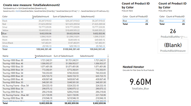
Viewing the two tables on the left, the totals sales for the Blue products for all methods is approximately 9.60M. Selecting the blue row in the top table filters the table below, to show sales by Product for only blue products. Viewing the totals for all three methods also shows a value of approximately 9.60M. Lastly, viewing the value card under Nested Iterator shows that the above created DAX expressions results in the same value of 9.60M.
Key concepts are highlighted in the above example
- Both
SUMXandFILTERcreate row context - The
FILTERfunction returns a virtual table which is a subset ofSalesOrderDetail SUMXreturns the sum of the row-by-row calculation of the sale amount- The table passed to
SUMXis the table that is returned by theFILTERfunction, this table only persists during the evaluation ofSUMX
As DAX expressions get longer and more complex formatting the expression will help make them easier to read and understand, tools such as DAXFormatter can aid in formatting
The concept of evaluation context has been mentioned in this post as well as in the previous post – Power BI Row Context: Understanding the Power of Context in Calculations.
Power BI Row Context: Understanding the Power of Context in Calculations
Row Context — What it is, When is it available, and its Implications
Evaluation context is the context in which a DAX formula evaluates a calculation. There are two types, Power BI Row Context: Understanding the Power of Context in Calculations explored the first type, row context. This post explored iterators or specific functions which create row context to perform multi-column calculations. Check out Part Three of this series which will explore the second type of evaluation context, the filter context.

Power BI Filter Context: Unraveling the Impact of Filters on Calculations
Filter Context – How to create it and its impact on measures
Thank you for reading! Stay curious, and until next time, happy learning.

And, remember, as Albert Einstein once said, “Anyone who has never made a mistake has never tried anything new.” So, don’t be afraid of making mistakes, practice makes perfect. Continuously experiment and explore new DAX functions, and challenge yourself with real-world data scenarios.
If this sparked your curiosity, keep that spark alive and check back frequently. Better yet, be sure not to miss a post by subscribing! With each new post comes an opportunity to learn something new.