
Subscribe to continue reading
Subscribe to get access to the rest of this post and other subscriber-only content.

Subscribe to get access to the rest of this post and other subscriber-only content.

Unlock the secrets to enhanced productivity and seamless project management.
In today’s fast-paced business environment, mastering the art of productivity is not just an option, but a necessity. The dynamic duo of Microsoft Planner and Power Automate are our allies in the realm of project and task management. Imagine a world where our projects flow seamlessly, where every task aligns perfectly with your goals, and efficiency is not just a buzzword but a daily reality. This is all achievable with the integrations of Microsoft Planner and Power Automate in your corner.
Microsoft Planner, is our go-to task management tool, that allows us and our teams to effortlessly create, assign, and monitor tasks. It provides a central hub where tasks aren’t just written down but are actively managed and collaborated on. Its strength lies in its visual organization of tasks, with dashboard and progress indicators providing an bird’s-eye view of our project, making organization and prioritization a breeze. It is about managing the chaos of to-dos into an organized methodology of productivity, with each task moving smoothly from To Do to Done.
On the other side of this partnership we have Power Automate, the powerhouse of process automation. It bridges the gap between our various applications and services, automating the mundane so we can focus on what is important. Power Automate is our behind the scenes tool for productivity, connecting our favorite apps and automating workflows whether that’s collecting data, managing notifications, sending approvals, and so much more all without us lifting a finger, after the initial setup of course.
Together, these tools don’t just manage tasks; they redefine the way we approach project management. They promise a future where deadlines are met with ease, collaboration is effortless, and productivity peaks are the norm.
Ready to transform your workday and elevate your productivity? Let Microsoft Planner and Power Automate streamline your task management.
Here’s an overview of what is explored within this post. Start with an overview of Power Automate triggers and actions specific to Microsoft Planner or jump right to some example workflows.
Exploring Planner triggers in Power Automate reveals a world of automation that streamlines task management and enhances productivity. Let’s dive into three key triggers and their functionalities.
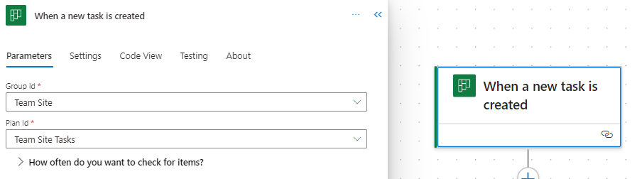
This trigger jumps into action as soon as a new task is created in Planner. It requires the Group Id and Plan Id to target the specific Planner board. This trigger can set a series of automated actions into motion, such as sending notifications to relevant team members, logging the task in an Excel reporting workbook, or triggering parallel tasks in a related project.
This trigger personalizes your task management experience. It activates when a task in Planner is assigned to you. This trigger can automate personal notifications, update your calendar with the new tasks, or prepare necessary documents or templates associated with the task. Simply select this Planner trigger and it is all set, there is no additional information required by the trigger. It’s an excellent way to stay on top of personal responsibilities and manage your workload efficiently.

The completion of a task in Planner can signal the start of various subsequent actions, hinging on the completion status of a task in a specified plan. The required inputs are the Group Id and the Plan Id to identify the target Planner board. This trigger is instrumental in automating post-task processes like updating project status reports, notifying team members or stakeholders of the task completion, or archiving task details for accountability and future reference.

By leveraging these Planner triggers in Power Automate, we can not only automate but also streamline our workflows. Each trigger offers a unique avenue to enhance productivity and ensures that our focus remains on strategic and high-value tasks.
Navigating the complexities of project management requires tools that offer both flexibility and control. The integration of Microsoft Planner actions within Power Automate provides a robust solution for managing tasks efficiently. By leveraging Planner actions in Power Automate, we can automate and refine our task management processes. Let’s dive into some of the different Planner actions.
Task assignment is a critical aspect of project management. These actions in Power Automate facilitate flexible and dynamic assignment and reassignment of team members to tasks in Planner, adapting to the ever-changing project landscape.
Add assignees to a task
This action allows us to assign team members to specific tasks, with inputs including the task ID and the user ID(s) of the assignee(s). It’s particularly useful for quickly adapting to changes in project scope or team availability, ensuring that tasks are always in the right hands.

Remove assignees from a task
Inputs for this action are the task ID and the user ID(s) of the assignee(s) to be removed. It’s essential for reorganizing task assignments when priorities shift or when team members need to be reallocated to different tasks, maintaining optimal efficiency.
The lifecycle of a task within any project involves its creation and eventual completion or removal. These actions in Power Automate streamline these essential stages, ensuring seamless task management within Planner.
Create a task
Every project begins with a single step, or in the case of our Planner board, a single task. To create a task we must provide the essentials, including Group Id, Plan Id, and Title. This action is invaluable for initiating tasks in response to various Power Automate triggers, such as email requests or meeting outcomes, ensuring timely task setup.

When using the new Power Automate designer (pictured above), be sure to provide all optional details of the task by exploring the Advanced parameters dropdown. Under the advanced parameters we will find task details to set in order to create a task specific to what our project requires. We can set the newly created task’s Bucket Id, Start Date Time, Due Date Time, Assigned User Id, as well as applying any tags needed to create a detailed and well defined task. When using the classic designer we will see all these options listed within the action block.
Delete a task
Keeping our Planner task list updated and relevant is equally important to successful project lifecycle management. Removing completed, outdated, or irrelevant tasks can help us maintain clarity and focus on the overall project plan. This action just requires us to provide the Task Id of the task we want deleted from our Planner board.
Accessing and updating task information are key aspects of maintaining project momentum. These actions provide the means to efficiently manage task within Planner.
Get a task
Understanding each task’s status is crucial for effective management, and the Get a task action offers a window into the life of any task in our Planner board. By providing the Task Id, this action fetches the task returning information about the specific task. It is vital for our workflows that require current information about a task’s status, priority, assignees, or other details before proceeding to subsequent steps. This insight is invaluable for keeping a pulse on our projects progress.

Update a task
This action, requires the Task Id and the task properties to be updated, allowing for real-time modifications of task properties. It is key for adapting tasks to new deadlines, changing assignees, or updating a task’s progress. Using this action we can ensure that our Planner board always reflects the most current state of our tasks providing a current overview of the overall project status.

Detailed task management is often necessary for complex projects. These actions cater to this need by providing and updating in-depth information about tasks in Planner.
Get task details
Each task in a project has its own story, filled with specific details and nuances. This action offers a comprehensive view of a task, including its description, checklist items, and more. It is an essential action for workflows that require a deep understanding of task specifics for reporting, analysis, or decision making.

Update task details
With inputs for detailed aspects of our tasks, such as its descriptions and checklist items, this action allows for precise and thorough updates to our task information. It is particularly useful for keeping tasks fully aligned with project developments and team discussions.

Effective task categorization is vital for clear project visualization and management. The List buckets action in Power Automate is designed to provide a comprehensive overview of task categories or buckets within our Planner board. We provide this action the Group Id and Plan Id and it returns a list of all the buckets within the specified plan, including details like bucket Id, name, and an order hint.
This information can aid in our subsequent actions, such as creating a new task within a specific bucket on our Planner board.

Keeping a tab on all tasks within a project is essential for effective project tracking, reporting, and management. The List tasks action in Power Automate offers a detailed view of tasks within a specific planner board.
We need to provide this action the Group Id and Plan Id, and it provides a detailed list of all tasks. The details provided for each task include the title, start date, due date, status, priority, how many active checklist items the task has, categories applied to the task, who created the task, and who the task is assigned to. This functionality is invaluable for teams to gain insights into task distribution, progress, and pending actions, ensuring that no task is overlooked and that project milestones are met.

Before diving into some more advanced examples and integrations, it is essential to understand how Planner and Power Automate can simplify everyday task management through some basic workflows. These workflows will provide a glimpse into the potential of combining these two powerful tools.
This workflow automates the process of summarizing completed tasks in Planner, sending a weekly email to project managers so they can keep their finger on the pulse of project progress.
The flow has a reoccurrence trigger which is set to run the workflow on a weekly basis. The workflow then starts by gathering all the tasks from the planner board using the List tasks action. This action provides two helpful task properties that we can use to pinpoint the task that have been completed in the last week.
The first is percentComplete, we add a filter data operation action to our workflow and filter to only tasks that have a percentComplete equal to 100 (i.e. are marked completed). We set the From input to the value output of the List task action and define our Filter Query.

The second property we can use from List tasks is the completedDateTime, we can use this to further filter our completed task to just those completed within the last week. Here we use the body of our Filter array: Completed tasks action and use an expression to calculated the difference between when the task was completed and when the flow is ran, in days.

The expression used in the filter query is:
int(split(dateDifference(startOfDay(getPastTime(1, 'Week')), item()?['completedDateTime']), '.')[0])
This expression starts by getting the start of the day 1 week ago using getPastTime and startOfDay. Then we calculate the difference using dateDifference. The date difference function will return a string value in the form of 7.00:00:00.0000000, representing Days.Hours:Minutes:Seconds. For our purposes we are only interested in the number of days, specifically whether the value is positive or negative, that is was it completed before or after the date 1 week ago. To extract just the days as an integer we first use split to split the string based on periods, and then we use the first item in the resulting array ([0]), and pass this to the int function, to get a final integer value.
We then use the Create HTML table action to create a summary table of the Planner tasks that were completed in the past week.

Then we can send out an email to those that require the weekly summary of completed tasks, using the output of the Create HTML table: Create summary table action.

Here is an overview of the entire Power Automate workflow that automates our process of summarizing our Planner tasks that have been completed in the past week.

This automated summary is invaluable for keeping track of progress and upcoming responsibilities, ensuring that our team is always aligned and informed about the week’s achievements and ready to plan for what is next.
This workflow is tailored to enhance team awareness and acknowledgement of completed high-priority tasks. It automatically sends a Teams notification when a high-priority task in Planner is marked as completed.
The workflow triggers when a Planner task on the specified board is marked complete. The workflow then examines the priority property of the task to determine if a notification should be sent. For the workflow a high-priority task is categorized as a task marked as Important or Urgent in Planner.

The workflow uses a condition flow control to evaluate each task’s priority property. An important note here is that, although in Planner the priorities are shown as Low, Medium, Important, and Urgent, the property values associated with these values are stored in the task property as 9, 5, 3, 1, respectively. So the condition used evaluates to true if the priority value is less than or equal to 3, that is the task is Important or Urgent.
When the condition is true, the workflow gathers more details about the task and then sends a notification to keep the team informed about these critical tasks.

Let’s break down the three actions used to compose and send the Teams notification. First, we use the List buckets action to provide a list of all the buckets contained within our Planner board. We need this to get the user friendly bucket name, because the task item only provides us the bucket id.
Then we can use use the Filter data operation to filter the list of all the buckets to the specific bucket the complete task resides in.

Here, value is the output of our List bucket action, id is the current bucket list item, and bucketId is the id of the current task item of the For each: Completed task loop. We can then use the dynamic content from the output of this action to provide a bit more detail to our Teams notification.
Now we can piece together helpful information and notify our team when high-priority tasks are completed using the Teams Post a message in a chat or channel action, shown above. Providing our team details like the task name, the bucket name, and a link to the Planner board.
These basic yet impactful workflows illustrate the seamless integration of Planner with Power Automate, setting the stage for more advanced and interconnected workflows. They highlight how simple automations can significantly enhance productivity and team communication.
The integration of Microsoft Planner with other services through Power Automate unlocks new dimensions in project management, offering innovative ways to manage tasks and enhance collaboration.
A standout application of this integration is the reporting of Planner tasks in Excel. By establishing a flow in Power Automate, task updates from Planner can be seamlessly merged to an Excel workbook. This setup is invaluable for generating detailed reports, tracking project progress, and providing more in-depth insights.
For an in-depth walkthrough of a workflow, leveraging this integration check out this post that covers the specifics of setting up and utilizing this integration.

Transforming Project Tracking: How to Merge Planner with Excel Using Power Automate
Explore the Detailed Workflow for Seamless Task Management and Enhanced Reporting Capabilities.
Combining Planner with GitHub through Power Automate creates a streamlined process for managing software development tasks. A key workflow in this integration is the generation of Planner tasks in response to new GitHub issues assigned to you. When an issue is reported in GitHub, a corresponding task is automatically created in Planner, complete with essential details from the GitHub issue. This integration ensures prompt attention to issues and their incorporation into the broader project management plan.
Check back, for a follow up post focus specifically on providing a detailed guide on implementing this workflow.
These advanced workflows exemplify the power and flexibility of integrating Planner with other services. By automating interactions across different platforms, teams can achieve greater efficiency and synergy in their project management practices.
Finishing our exploration of Microsoft Planner and Power Automate, it’s evident that these tools are more than mere facilitators of task management and workflow automation. They embody a transformative approach to project management, blending efficiency, collaboration, and innovation in a unique and powerful way.
The synergy between Planner and Power Automate opens up a realm of possibilities, enabling teams and individuals to streamline their workflows, integrate with a variety of services, and automate processes in ways that were previously unimaginable. From basic task management to complex, cross-platform integrations with services like Excel and GitHub, these tools offer a comprehensive solution to the challenges of modern project management.
The journey through the functionalities of Planner and Power Automate is a testament to the ever-evolving landscape of digital tools and their impact on our work lives. As these tools continue to evolve, they offer fresh opportunities for enhancing productivity, fostering team collaboration, and driving innovative project management strategies.
Experiment with these tools and explore the myriad of features they have to offer, and discover new ways to optimize your workflows. The combination of Planner and Power Automate isn’t just a method for managing tasks; it’s a pathway to redefining project management in the digital age, empowering teams to achieve greater success and efficiency.
Thank you for reading! Stay curious, and until next time, happy learning.

And, remember, as Albert Einstein once said, “Anyone who has never made a mistake has never tried anything new.” So, don’t be afraid of making mistakes, practice makes perfect. Continuously experiment, explore, and challenge yourself with real-world scenarios.
If this sparked your curiosity, keep that spark alive and check back frequently. Better yet, be sure not to miss a post by subscribing! With each new post comes an opportunity to learn something new.

Elevate Your Power BI Reports with Context-Aware Insights
Welcome, to another journey through the world of DAX, in this post we will be shining the spotlight on the ISINSCOPE function. If you have been exploring DAX and Power BI you may have encountered this function and wondered its purpose. Well, wonder no more! We are here to unravel the mysteries and dive into some practical example showing just how invaluable this function can be in our data analysis endeavors.
If you are unfamiliar DAX is the key that helps us unlock meaningful insights. It is the tool that lets us create custom calculations and serve up exactly what we need. Now, lets focus on ISINSCOPE, it is a function that might not always steal the show but plays a pivotal role, particularly when we are dealing with hierarchies and intricate drilldowns in our reports. It provides us the access to understand at which level of hierarchy our data is hanging out, ensuring our calculations are always in tune with the context.
For those of you eager to start experimenting there is a Power BI report pre-loaded with the sample data used in this post ready for you. So don’t just read, follow along and get hands-on with DAX in Power BI. Get a copy of the sample data file (power-bi-sample-data.pbix) here:

GitHub – Power BI DAX Function Series: Mastering Data Analysis
This dynamic repository is the perfect place to enhance your learning journey.
Let’s dive in and get hand on with the ISINSCOPE function. Think of this function as our data GPS, it helps us figure out where we are in the grand scheme of our data hierarchies.
So, what exactly is ISINSCOPE? In plain terms, it is a DAX function used to determine if a column is currently being used in a specific level of a hierarchy or, put another way, if we are grouping by the column we specify. The function returns true when the specified column is the level being used in a hierarchy of levels. The syntax is straightforward:
ISINSCOPE(column_name)
The column_name argument is the name of an existing column. Just add a column that we are curious about, and ISINSCOPE will return true or false depending on whether that column is in the current scope.
Let’s use a simple matrix containing our Region, Product Category, and Product Code to set up a hierarchy and see ISINSCOPE in action with the following formula.
ISINSCOPE =
SWITCH(
    TRUE(),
    ISINSCOPE(Products[Product Code]), "Product Code",
    ISINSCOPE(Products[Product]), "Product",
    ISINSCOPE(Regions[Region]), "Region"
)
This formula uses ISINSCOPE in combination with SWITCH to determine the current context, and if true returns a text label indicating what level is in context.

But why is this important? Well, when we are dealing with data, especially in a report or a dashboard, we want our calculations to be context-aware. We want them to adapt based on the level of data we are looking at. ISINSCOPE allows us to create measures and calculated columns that behave differently at different levels of granularity. This helps provide accurate and meaningful insights.
Now that we have got a handle on what ISINSCOPE is, let’s dive a bit deeper and see how it works. At the heart of it ISINSCOPE is all about context, specifically, row context and filter context.
For an in depth look into Row Context and Filter Context check out the posts below that provide all the details.

Power BI Row Context: Understanding the Power of Context in Calculations
Row Context — What it is, When is it available, and its Implications

Power BI Filter Context: Unraveling the Impact of Filters on Calculations
Filter Context – How to create it and its impact on measures
For our report we are interested in analyzing the last sales date of our products, and want this information in a matrix similar to the example above. We can easily create a Last Sales Date measure using the following formula and add it to our matrix visual.
Last Sales Date = MAX(Sales[SalesDate])

This provides a good start, but not quite what we are looking for. For our analysis the last sales date at the Region level is too broad and not of interest, while the sales date of Product Code is too granular and clutters the visual. So, how do we display the last sales date just at the Product Category (e.g. Laptop) level? Enter ISINSCOPE.
Let’s update our Last Sales Date measure so that it will only display the date on the product category level. Here is the formula.
Product Last Sales Date =
SWITCH(
    TRUE(),
    ISINSCOPE(Products[Product Code]), BLANK(),
    ISINSCOPE(Products[Product]), FORMAT(MAX(Sales[SalesDate]),"MM/dd/yyyy"),
    ISINSCOPE(Regions[Region]), BLANK()
)

We use SWITCH in tandem with ISINSCOPE to determine the context, and if Product is in context the measure returns the last sales date for that product category. However, at the Region and Product Code levels the measure will return a blank value.
The use of ISINSCOPE helps enhance the matrix visual preventing it from getting over crowded with information and ensuring that the information displayed is relevant. It acts as a smart filter, showing or hiding data based on where we are in a hierarchy, making our reports more intuitive and user-friendly.
When we are working with data, understanding the relationship between parts and the whole is crucial. This is where hierarchies and drilldowns come into play, and ISINSCOPE is the function that helps us make sense of it all.
Hierarchies allow us to organize our data in a way that reflects real-world relationships, like breaking down sales by region, then product category, then specific products. Drilldowns let us start with a broad view and then zoom in on the details. But how do we keep our calculations accurate at each level? You guessed it, ISINSCOPE.
Let’s look at a DAX measure that leverages ISINSCOPE to calculate the percentage of sales each child represents of the parent in our hierarchy.
Percentage of Parent =
    VAR AllSales =
        CALCULATE(Sales[Total Sales], ALLSELECTED())
    VAR RegionSales =
        CALCULATE([Total Sales], ALLSELECTED(), VALUES(Regions[Region]))
    VAR RegionCategorySales =
        CALCULATE([Total Sales], ALLSELECTED(), VALUES(Regions[Region]), VALUES(Products[Product]))
    VAR CurrentSales = [Total Sales]

RETURN
SWITCH(TRUE(),
    ISINSCOPE(Products[Product Code]), DIVIDE(CurrentSales, RegionCategorySales),
    ISINSCOPE(Products[Product]), DIVIDE(CurrentSales, RegionSales),
    ISINSCOPE(Regions[Region]), DIVIDE(CurrentSales, AllSales)
)
The Percentage of Parent measure uses ISINSCOPE to determine the current level of detail we are working with. If we are viewing our sales by region the measure calculates the sales for the region as a percentage of all sales.

But the true power of ISINSCOPE begins to reveal itself as we drilldown into our sales data. If we drilldown into each region to show the product categories we see that the measure will calculate the sales for each product category as a percentage of sales for that region.

And then again, if we drilldown into each product category we can see the measure will calculate the the sales of each product code as a percentage of sales for that product category within the region.

By incorporating this measure into our report, we help ensure that as we drilldown into our data the percentages are always calculated relative to the appropriate parent in our hierarchy. This allows us to provide accurate measures that provide the appropriate context, making our reports more intuitive and insightful.
ISINSCOPE is the key element to maintaining the integrity of our hierarchical calculations. It ensures that as we navigate through different levels of our data our calculations remain relevant and precise, providing a clear understanding of how each part contributes to the whole.
When it comes to DAX and ISINSCOPE a few best practices can ensure that our reports are accurate, performant, and user-friendly. Here are just a few things that can help us make the most out of ISINSCOPE:
ISINSCOPE, make sure to have a solid understanding of row and filter context. Knowing which context we are working with will help us use ISINSCOPE effectively.ISINSCOPE behaves with our data. Complex measures can be built up gradually as we become more comfortable with the function.ISINSCOPE, test them at every level, this helps ensure that our measures work correctly no matter how the users interact with the report.ISINSCOPE is often used in combination with other DAX functions. Learning how it interacts with functions like SWITCH, CALCULATE, FILTER, and ALLSELECTED will provide us more control over our data.Throughout our exploration of the ISINSCOPE function we have uncovered its pivotal role in managing data hierarchies and drilldowns providing for accurate and context-sensitive reporting. Its ability to discern the level of detail we are working with allows for dynamic measures and visuals that adapt to user interactions, making our reports not just informative but interactive and intuitive.
With practice, ISINSCOPE will become a natural part of your DAX toolkit, enabling you to create sophisticated reports that meet the complex needs of any data analysis challenge you might face.
For those looking to continue their journey into DAX and its capabilities there is a wealth of resources available, and a good place to start is the DAX Reference documentation.

Excel Online (Business) – Actions
Learn more about: Power Automate Excel Online (Business) Actions
I have also written about other DAX functions including Date and Time Functions, Text Functions, an entire post focused on the CALCULATE function and an ultimate guide providing a overview of all the DAX function groups.

Temporal Triumphs with DAX Date and Time Functions
Explore the ebb and flow of the temporal dimension of your data with DAX’s suite of Date and Time Functions.

Mastering DAX Text Expressions: Making Sense of Your Data One String at a Time
Stringing Along with DAX: Dive Deep into Text Expressions

Unlocking the Secrets of CALCULATE: A Deep Dive into Advanced Data Analysis in Power BI
Demystifying CALCULATE: An exploration of advanced data manipulation.

The DAX Function Universe: A Guide to Navigating the Data Analysis Tool box
Unlock the Full Potential of Your Data with DAX: From Basic Aggregations to Advanced Time Intelligence
Thank you for reading! Stay curious, and until next time, happy learning.
And, remember, as Albert Einstein once said, “Anyone who has never made a mistake has never tried anything new.” So, don’t be afraid of making mistakes, practice makes perfect. Continuously experiment and explore new DAX functions, and challenge yourself with real-world data scenarios.
If this sparked your curiosity, keep that spark alive and check back frequently. Better yet, be sure not to miss a post by subscribing! With each new post comes an opportunity to learn something new.

Explore the ebb and flow of the temporal dimension of your data with DAX’s suite of Date and Time Functions.
In data analysis, understanding the nuances of time can be the difference between a good analysis and a great one. Time-based data, with its intricate patterns and sequences offers a unique perspective into trends, behaviors, and potential future outcomes. DAX provides specialized date and time functions helping guide us through the complexities of temporal data with ease.
Curious what this post will cover? Here is the break down, read top to bottom or jump right to the part you are most interested in.
For those of you eager to start experimenting there is a Power BI report pre-loaded with the sample data used in this post ready for you. So don’t just read, following along and get hands-on with DAX in Power BI. Get a copy of sample data file (power-bi-sample-data.pbix) here:

GitHub – Power BI DAX Function Series: Mastering Data Analysis
This dynamic repository is the perfect place to enhance your learning journey and serves as an interactive compliment to the blog posts on EthanGuyant.com.
Consider the role of a sales manager for a electronic store. Knowing 1,000 smartphones were sold last month provides a good snapshot. But, understanding the distribution of these sales-like the surge during weekends or the lull on weekdays-offers greater insights. This level of detail is made possible by time-based data and allows for more informed decisions and strategies.
For many, the journey into DAX begins with a foundation in Excel and the formulas it provides. While DAX and Excel share a common lineage, they two have distinct personalities and strengths. Throughout this post if you are familiar with Excel you may recognize some functions but it is important to note that Excel and DAX work with dates differently.
Both DAX and Excel boast a rich array of functions, many of which sound and look familiar. For instance the TODAY() function exists in both. In Excel, TODAY() simply returns the current date. In DAX, while TODAY() also returns the current date it does so within the context of the underlying data model, allowing for more complex interactions and relationships with other data in Power BI.
Excel sees dates and times as serial numbers, a legacy of its spreadsheet origins. DAX, on the other hand, elevates them with a datetime data type. This distinction means that in DAX, dates and times are not just values, they are entities with relationships, hierarchies, and attributes. This depth allows for a range of calculations in DAX that would require workarounds in Excel. And with DAX’s expansive library of date time functions, the possibilities are vast.
For more details on DAX date and time functions keep reading and don’t forget to also checkout the Microsoft documentation.
Learn more about: Date and time functions
Diving into DAX can fell like like stepping into the ocean. But fear not! Let’s wade into the shallows first by getting familiar with some basic functions. These foundational functions will set the stage for more advanced explorations later on.
The DATE function in DAX is a tool for manually creating dates. It syntax is:
DATE(year, month, day)
As you might expect, year is a number representing the year. What may not be as clear is the year argument can include one to four digits. Although years can be specified with two digits it best practice to use four digits whenever possible to avoid unintended results. For example:
Use Four Digit Years = DATE(23, 1, 1)
Will return January 1st, 1923, not January 1st, 2023 as may have been intended.

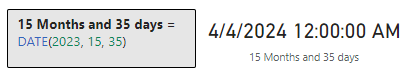
The month argument is a number representing the month, if the value is a number from 1 to 12 then it represents the month of the year (1-January, …, 12-December). However, if the value is greater than 12 a calculation occurs. The date is calculated by adding the value of month to January of the specified year. For example, using DATE if we specify the year as 2023 and the month as 15, we will get a results for March 2024.
15 Months = DATE(2023, 15, 1)

Similarly the argument day is a number representing the day of the month or a calculation. The day argument results in a calculation if the value is greater than the last day of the given month, otherwise it simply represents the day of the month. The calculation is similar to how the month argument works, if day is greater than the last day of the month the value is added to month. If we take the example above and change day to be 35, we can see it returns a date of April 4th, 2024.
Sometimes, we just need a piece of the date. Whether it is the day, month, or year, DAX has a function for that. All of these functions have similar syntax and have a singular date argument which can be a date in datetime format or text format (e.g. “2023-01-01”).
DAY(date)
MONTH(date)
YEAR(date)

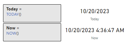
Note: At the time of writing today is 10/20/2023. The TODAY() function is used through out this post.
These functions are pivotal when segmenting data, creating custom date hierarchies, or performing year-over-year and month-over-month analyses.
In the dynamic realm of data, real-time insights are invaluable. The TODAY function in DAX delivers the current date without time details. It is perfect for age calculations or determining days since a particular event. Conversely, NOW provides a detailed timestamp, including the current time. This granularity is essential for monitoring live data, event logging, or tracking activities.
The examples above provide examples of using TODAY, the below example highlights the differences between TODAY and NOW.
With these foundational date functions in our tool box we are equipped to continue deeper into DAX’s date and time capabilities. These might seem basic, but their adaptability and functionality are the bedrock for more complex and advanced operations and analyses.
As we become more comfortable with DAX’s basic date functions you may begin to wonder what more can DAX’s Date and Time functions do. Diving deeper into DAX’s date functions we will discover more advanced tools specific to addressing date-related challenges. Whether it is shifting dates, pinpointing specific moments, or calculating intervals, DAX’s date and time functions are here to elevate our data analysis and conquer these challenges.
A common challenge we may encounter is the need to project a date a few months into the future or trace back to a few months prior. EDATE is the function for the job, EDATE allows us to shift a date by a specified number of months. The syntax is:
EDATE(start_date, months)
The start_date is a date in datetime or text format and is the date that we want to shift by the value of months. The months argument is an integer representing the number of months before or after the start_date. One thing to note is that if the start_date is provided in text format the function will interpret this based on the locale and date time settings of the client computer. For example if start_date is 10/1/2023 and the date time settings represent a date as Month/Day/Year this will be interpreted as October 1st, 2023, however if the date time settings represent a date as Day/Month/Year it will be interpreted as January 10th, 2023.
For example, say we follow up on a sale or have a business process that kicks off 3 months following a sale. We can use EDATE to project the SalesDate and identify when this process should occur. We can use:
3 Months after Sale = EDATE(MAX(Sales[SalesDate]), 3)

End-of-month dates are crucial for a variety of purposes. With EOMONTH we can easily determine the last date of a month. The syntax is the same as EMONTH:
EOMONTH(start_date, months)
We can use this function to identify the end of the month for each of our sales.
Sales End of Month = EOMONTH(MAX(Sales[SalesDate]), 0)

In the example above we use 0 to indicate we want the end of the month in which the sale occurred. If we needed to project the date to the end of the following month we would update the months argument from 0 to 1.
The temporal aspects of our data can be so much more than static points on a timeline. They can represent intervals, durations, and sequences. By understanding the span between dates or manipulating these intervals we can provide additional insights required by our analysis.
DATEDIFF is the function to use when measuring the span between two dates. With this function we can calculate the age of an item, or the duration of a project. DATEDIFF calculates the difference between the dates base on days, months, or years. Its syntax is:
DATEDIFF(date_1, date_2, interval)
The date_1 and date_2 arguments are the two dates that we want to calculated the difference between. The result will be a positive value if date_2 is larger than date_1, otherwise it will return a negative result. The interval argument is the interval to use when comparing the two dates and can be SECOND, MINUTE, HOUR, DAY, WEEK, MONTH, QUARTER, or YEAR.
We can use DATEDIFF and the following formula to calculate how many days it has been since our last sale, or the difference between our last Sales date and Today.
Days Between Last Sale and Today =
DATEDIFF(MAX(Sales[SalesDate]), TODAY(), DAY)

The above example shows as of 10/20/2023 it has been 64 days since our last sale.
In the DATE: Crafting Dates in Datetime Format section we saw that providing DATE a month value greater than 12 or a day value greater than the last day of the month will add values to the year or month. However, if the goal is to adjust our dates by an specific interval the DATEADD function can be much more useful. Although in the DAX Reference documentation DATEADD is categorized under Time Intelligence functions it is still helpful to mention here. The syntax for DATEADD is:
DATEADD(dates, number_of_intervals, interval)
The dates argument is a column that contains dates. The number_of_intervals is an integer that specifies the number of intervals to add or subtract. If number_of_intervals is positive the calculation will add the intervals to dates and if negative it will subtract the intervals from dates. Lastly, interval is the interval to adjust the dates by and can be day, month, quarter, or year. For more details and examples on DATEADD checkout my previous post Time Travel in Power BI: Mastering Time Intelligence Functions.

Time Travel in Power BI: Mastering Time Intelligence Functions
Journey through the Past, Present, and Future of Your Data with Time Intelligence Functions.
Advanced date manipulations in DAX open up a world of possibilities. From forecasting and backtracking to pinpointing specific intervals. These functions empower us to navigate the intricacies of our data providing clarity and depth to our analysis.
In data analysis, time is so much more than just ticking seconds on a clock. Time provides an element of our data to help understand its patterns looking back, or predicting trends looking forward. DAX provides us a suite of time functions that allow us to dissect, analyze, and manipulate time data.
Time is a composite of hours, minute, and seconds. DAX provides individual functions that extract each of these components.
As you might have expected these functions are appropriately named HOUR, MINUTE, and SECOND. They also all follow the same general syntax.
HOUR(datetime)
MINUTE(datetime)
SECOND(datetime)
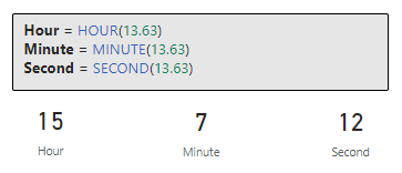
Each function then returns its respective time component, HOUR will return a value from 0 (12:00AM) to 23 (11:00PM), MINUTE returns a value from 0 to 59, and SECOND returns a value also from 0 to 59.
All of these functions take the datetime that contains the component we want to extract as the singular argument. The time can be supplied using datetime format, another expression that returns a datetime (e.g. NOW()), or text in an accepted time format. When the datetime is provided as text the function uses the locale and datetime setting of the client computer to interpret the text value. Most locales use a colon : as the time separator and any text input using colons will parse correctly.

It is also important to be mindful when these functions are provided a numeric value to avoid unintended results. The serial number will first be represented as a datetime data type before the time component is extracted. To more easily understand the results of our calculations its best to first represent these values as datetime data types before passing them to the functions. For example, passing a value of 13.63 to the HOUR function will return a value of 15. This is because 13.63 is first represented as a datetime 1/13/1900 15:07:12 and then the time components are extracted.
In our datasets time values might sometimes be stored as text. The TIMEVALUE function is the go to tool for handling these text values. This function will convert a text representation of time (e.g. "18:15") into a time value. Applying TIMEVALUE converts the text to a time value making it usable for time-based calculations.
Text to Time = TIMEVALUE("18:15")

DAX’s time functions allow us to zero in on the details of our datetime data. When we need to segment data by hours, set benchmarks, or convert time formats, these functions ensure we always have the tools ready to address these challenges.
Dates and times a crucial parts of many analytical tasks. DAX offers a wide array of specialized functions that cater to unique date and time requirements helping us ensure we have the proper tools needed for every analytical challenge we face.
When developing our data model having a continuous date table can be an invaluable asset. DAX provides two functions that can help us generate date table within our data model.
CALENDAR will create a table with a single “Date” column containing a contiguous set of dates starting from a specified start date and ending at a specified end date. The syntax is:
CALENDAR(start_date, end_date)
The range of dates is specified by the two arguments and is inclusive of these two dates. CALENDAR will result in an error if start_date is greater than end_date.
CALENDARAUTO takes CALENDAR one step further by adding some automation. This function will generate a date table based on the data already in our data model. It identifies the earliest and latest dates and creates a continuous date table accordingly. When using CALENDARAUTO we do not have to manually specify the start and end date, here is the functions syntax:
CALENDARAUTO([fiscal_year_end_month])
The CALENDARAUTO function has a single optional argument fiscal_year_end_month. This argument can be used to specify the month the year ends and can be a value from 1 to 12. If omitted the default value will be 12.
A few things to note about the automated calculation. The start and end dates are determined by dates in the data model that are not in a calculated column or a calculated table and the function will generate an error if no datetime values are identified in the data model.
In business scenarios, understanding workdays is crucial for tasks like planning or financial forecasting. The NETWORKDAYS functions calculates the number of whole workdays between two dates, excluding weekends and providing the options to exclude holidays. The syntax is:
NETWORKDAYS(start_date, end_date[, weekend, holidays])
The start_date and end_date are the dates we want to know how many workdays are between. Within the NETWORKDAYS the start_date can be earlier than, the same as, or later than the end_date. If start_date is greater than end_date the function will return a negative value. The weekend argument is optional and is a weekend number which specifies when the weekends occur, for example a value of 1 (or if omitted) indicates the weekend days are Saturday and Sunday. Check out the parameter details for a list of all the options.
NETWORKDAYS function (DAX) – DAX | Parameters
Learn more about: NETWORKDAYS
Lastly, holidays is a column table of one or more dates that are to be excluded from the working day calendar.
Let’s take a look at an example, from our previous Days Between Last Sale and Today example we know there at 64 days since our last sale. Let’s use the following formula to identify how many of those are workdays.
Workday Between Last Sale and Today =
NETWORKDAYS(MAX(Sales[SalesDate]), [Today], 1)
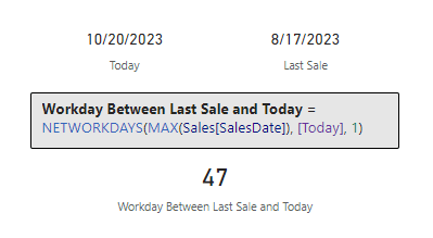
Note: At the time of writing the last sales date is 8/17/2023 and today is 10/20/2023
Taking into account the date range noted above, we can update the Workday Between Last Sale and Today to exclude Labor Day (9/4/2023) using this updated formula.
Workday Between Last Sale and Today (No Holidays) =
NETWORKDAYS(
    MAX(Sales[SalesDate]),
    [Today],
    1,
    {DATE (2023, 9, 4)}
)

When we need to categorized our dates into broader hierarchies functions like QUARTER and WEEKDAY can help with this task. QUARTER returns the quarter of the specified date and returns a number from 1 to 4.
QUARTER(date)

WEEKDAY provides the day number of the week ranging from 1(Sunday) to 7 (Saturday) by default.
WEEKDAY(date, return_type)
The date argument should be in datetime format and entered by using the DATE function or by another expression which returns a date. The return_type determines what value is returned, a value of 1 (or omitted) indicates the week begins on Sunday (1) and ends Saturday (7), 2 indicates the week begins Monday (1) and ends Sunday (7), and 3 the week begins Monday (0) and ends Sunday (6).
Let’s take a look at the WEEKDAY function and return_type by using the following formulas to evaluate Monday, 10/16/2023.
Weekday (1) = WEEKDAY(DATE(2023, 10, 16))
Weekday (2) = WEEKDAY(DATE(2023, 10, 16), 2)
Weekday (3) = WEEKDAY(DATE(2023, 10, 16), 3)

DAX’s specialized date and time functions are helpful tools designed just for us. They cater to the unique requirements of working with date and times, ensuring that we are set to tackle any analytical challenge we may face with precision and efficiency.
The annual cycle holds significance in numerous domains, from finance to academia. Yearly reviews, forecasts, and analyses form the cornerstone of many decision-making processes. DAX offers a set of functions to extract and manipulate year-related data, ensuring you have a comprehensive view of annual trends and patterns.
We have already explored the first function that provides yearly insights, YEAR. This straightforward yet powerful function extracts the year from a given date and allows us to categorize or filter data based on the year. Let’s explore some other DAX functions that help provide us yearly insights into our data.
Sometimes, understanding the fraction of a year between two dates can be beneficial. The YEARFRAC function calculates the fraction of a year between two dates. The syntax is:
YEARFRAC(start_date, end_date[, basis])
Same as other date functions start_date and end_date are the dates we are interested in knowing the fraction of a year between and they are passed to YEARFRAC in datetime format. The basis argument is optional and is the type of day count basis to be used for the calculation. The default value is 0 and indicates the use of US (NASD) 30/360. Other options include 1-actual/actual, 2-actual/360, 3-actual/365, and 4-European 30/360.
Let’s examine the difference between our last sale and today again. From our previous calculation we know there is 64 days between our last sale and today (10/23/2023), we can use YEARFRAC to represent this difference as a fraction of a year.
Fraction of Year Between Last Sale and Today =
YEARFRAC(MAX(Sales[SalesDate]), TODAY(), 0)

Our analysis in many scenarios may require or benefit from understanding weekly cycles. The WEEKNUM function gives us the week number of the specified date, helping us analyze data on a weekly basis. The syntax for WEEKNUM is
WEEKNUM(date[, return_type])
The return_type argument is optional and represents which day the week begins. The default value is 1 indicating the week begins on Sunday.
An important note about WEEKNUM is that the function uses a calendar convention in which the week that contains January 1st is considered to be the first week of the year. However, the ISO 8601 calendar standard defines the first week as the one that has four or more days (contains the first Thursday) in the new year, if this standard should be used the return_type should be set to 21. Check out the Remarks section of the DAX Reference for details on available options.
WEEKNUM function (DAX) – DAX | Remarks
Learn more about: WEEKNUM
Let’s explore the differences between using the default return_type where week one is the week which contains January 1st, and a return_type of 21 where week one is the first week that has four or more days in it (with the week starting on Monday). To do this we will fast forward to Wednesday January 6th, 2027.
In 2027 January 1st lands on a Friday, so using Monday as the start of the week results in 3 days in 2027 being in that week and the first week in 2027 with four or more days (or containing the first Thursday) begins Monday, January 4th.

Harnessing the power of these functions allows us to dive deep into annual trends, make better predictions, and craft strategies that resonate with the yearly ebb and flow of our data.
Time is a foundational element in data analysis. From understanding past trends to predicting future outcomes, the way we interpret and manipulate time data can significantly influence our insights. DAX offers a robust suite of date and time functions, providing a comprehensive toolkit to navigate the temporal dimensions of our data.
As business continue to trend toward being more data-driven, the need for precise time-based calculations will continue to grow. Whether it is segmenting sales data by quarters, forecasting inventory based on past trends, or understanding productivity across different time zones, DAX provides us the tools to tackle these tasks.
For those looking to continue this journey into DAX and its capabilities there is a wealth of resources available, and a good place to start is the DAX Reference documentation.
Excel Online (Business) – Actions
Learn more about: Power Automate Excel Online (Business) Actions
I have also written about other DAX function groups including Time Intelligence functions, Text Functions, an entire post focused on CALCULATE and an ultimate guide providing a overview of all the DAX function groups.
Time Travel in Power BI: Mastering Time Intelligence Functions
Journey through the Past, Present, and Future of Your Data with Time Intelligence Functions.
Mastering DAX Text Expressions: Making Sense of Your Data One String at a Time
Stringing Along with DAX: Dive Deep into Text Expressions
Unlocking the Secrets of CALCULATE: A Deep Dive into Advanced Data Analysis in Power BI
Demystifying CALCULATE: An exploration of advanced data manipulation.
The DAX Function Universe: A Guide to Navigating the Data Analysis Tool box
Unlock the Full Potential of Your Data with DAX: From Basic Aggregations to Advanced Time Intelligence
In the end, dates are more than just numbers on a calendar and time is more than just ticks on a clock. They are the keys to reveal the story of our data. With the power of DAX Date and Time Functions we will be able to tell this story with ease and in the most compelling way possible.
Thank you for reading! Stay curious, and until next time, happy learning.
And, remember, as Albert Einstein once said, “Anyone who has never made a mistake has never tried anything new.” So, don’t be afraid of making mistakes, practice makes perfect. Continuously experiment and explore new DAX functions, and challenge yourself with real-world data scenarios.
If this sparked your curiosity, keep that spark alive and check back frequently. Better yet, be sure not to miss a post by subscribing! With each new post comes an opportunity to learn something new.

Subscribe to get access to the rest of this post and other subscriber-only content.
