Chart your data journey! Transform data into insights with Power BI core visualizations.
Pie, Donut, and Treemap charts can be helpful tools when we need to show how different parts contribute to a whole. Pie charts represent data as slices of a circle and show the relationship of parts to a whole. Donut charts are similar to pie charts. However, their center is blank, providing space to add a label or other icon. Treemap charts use nested rectangles to visualize each level of hierarchy in our data.
These charts can be helpful for specific visualizations, but it is important to recognize their limitations. As with all of our data visualization tasks, choosing the right type of visual is essential. To explore bar and column charts, visit Part #1 of this series, and to learn more about line and area charts, check out Part #2.

Explore Power BI Core Visualizations: Part 1 – Bar and Column Charts
Chart your data journey! Transform data into insights with Power BI core visualizations.

Explore Power BI Core Visualizations: Part 2 – Line and Area Charts
Chart your data journey! Transform data into insights with Power BI core visualizations.
Customizing Pie Charts
Customizing our pie charts enhances their clarity, making it easier for our report viewers to interpret the data.
Adjusting Colors
The color choices used in our pie charts play a crucial role in their readability. Within the Slices property of our Pie chart, we can customize the colors used for each slice. When selecting colors, we should ensure they are visually distinct and that the colors used for our data categories are consistent across all visuals on the page and within the report.
We set the color of our slices in the Format pane, under the slices section. Here, we will find each data category included in the chart, and we can explicitly see the color.

Formatting Data Labels
The data labels on our pie charts help convey important insights to our viewers. Within the Data label properties of our pie chart we find several options to edit and format our data labels. We have options to set the position of our data labels (e.g. outside, prefer inside), what information to display such as category name, values, or percent of total, and under the Value grouping, we can format the text of the data labels.

Using a combination of these properties, we can make our charts more informative at a glance. For example, we can improve the above plot by displaying the category name and percent of total directly on our chart.

It is important to be cautious when using data labels. We want to provide essential information without overcrowding the chart with too much text. Adjusting the font size, background, font color, and label position can help us maintain a clean and organized look.
Using Legends Effectively
Our data labels display information directly on our charts, while legends offer a clean way to display what data category corresponds to which chart slice. Within the Legend properties we can set the position of the legend, set the title, and format the text and title of the legend.
We can update the Pie chart above to display the legend and then update the data label to display the total sales value and the percent of total value.

When using pie charts, it is important to limit the number of categories to ensure clarity. Pie charts are most effective when displaying data with no more than a few slices. If this cannot be accomplished, it’s best to consider other visuals to provide our insights.
Customizing Donut Charts
Donut charts provide an alternative to pie charts, with the added benefit of a central blank space. This space can be used for a variety of purposes or left blank. By customizing our donut charts, we can enhance their effectiveness and make them more informative and engaging.
Like pie charts, donut charts allow us to set the color of each chart slice, use data labels to provide additional information and position the legend to provide additional context.
Donut charts also offer additional properties we can customize to enhance these charts even further.
Modifying the Inner Radius
One of the main differences between our pie and donut charts is the open area in the center. Within the Slices property grouping, we will find a Spacing option. Here, we can adjust the inner radius, controlling how wide or narrow the chart’s ring appears.
Increasing this value creates a more pronounced donut shape, which can help draw viewers’ attention to the center of the chart. Decreasing this value makes the chart look more like a traditional pie chart.

Donut charts can be helpful when we need to compare proportions while also displaying an aggregate metric that we can place in the open center of the visual. However, like pie charts it is important to only use these charts when there is a small and manageable number of segments. When there are too many segments, donut and pie charts become cluttered and difficult to interpret.
When using these comparison charts, we should aim for simplicity and clarity.
Customizing Treemap Charts
Treemap charts are useful when visualizing hierarchical data. They allow us to display a large amount of information in a compact space. Each category in the visual is represented by a rectangle, the size of which reflects the category’s value.
Treemap charts offer various properties that we can customize to enhance their clarity, ensuring they effectively convey complex data structures and insights.
Adjusting the Colors
In our treemap visuals, colors distinguish between our different categories. Like in our other charts, we can set the color for each category, and it is important that this color selection is consistent across all visuals within our report. For example, we can create a treemap of our Total Sales by product category and product code and set the colors for each category to ensure visual consistency.

Setting Labels and Viewing Tooltips
Like many of our other Power BI visuals, Treemap visuals allow us to customize visual labels and tooltip properties to improve the readability of our visuals. Labels on our visuals provide context by displaying category names and values directly within each rectangle. By using the options available under the data labels and categories labels we can adjust the font size, color, display units, and the number of decimal places to improve the clarity of our visual.
We will use these properties to improve the treemap above by increasing the font size and weight of the category labels so they are easily identifiable. We will also turn on data labels to provide our viewers with precise information for the largest contributors.

Tooltips are another feature common across our Power BI visuals that adds an interactive element to our reports and can provide our viewers with additional information. When a user hovers over a rectangle, a tooltip appears, providing them with information about that category. Additionally, the information included within the tooltip can be customized to provide further context, such as percentages or other metrics.
In treemaps, some rectangles may be too small to display the data label, and tooltips become a valuable asset for delivering details without cluttering the visual.

Using Drill-Down Features
One strength of treemaps is their ability to represent hierarchical data. Power BI’s drill-down functionality lets us explore these hierarchies in detail. A user can use the drill-down feature to drill into the next level of the hierarchy, focusing on the subcategories or finer details of the data.
Drill-down features provide our viewers with another interactive element, allowing them to explore the dataset at multiple levels without overwhelming them with too much information upfront.
In our example treemap above, the first-level category is Product, and the second is Region. This allows our viewers to drill into a product category to view the distribution of product sales across sales regions.

Treemap charts can be a helpful tool for comparing proportions within hierarchical data. However, they are most effective when the differences in value between categories are significant. When all categories are similar in size, the visual can be difficult to interpret, so it is important to evaluate whether a treemap is appropriate for each use case.
Advanced Techniques and Customizations
Current Year Sales by Product Selection
The Current Year Sales donut chart helps visualize how a selected product contributes to the total current year sales.

To build this visual, we first, create two measures: Total Sales CY and Remaining CY Sales.
The Total Sales CY measure calculates the current year’s total sales, and the Remaining CY Sales calculates the difference between the total sales of all products and the selected product’s sales.
Total Sales CY = TOTALYTD([Total Sales], DateTable[Date])Remaining CY Sales =
VAR _allSales = CALCULATE([Total Sales CY], ALL(Sales))
RETURN
_allSales - [Total Sales CY]We then add these two measures to our donut chart’s Values property and set the color of the Total Sales CY to a dark blue and Remaining CY Sales to a light gray.

We then turn off the legend, and update the data labels to show only the percent of total value.
Next, we create a new measure that will be used for the visual subtitle. The subtitle provides additional context by showing how close the product’s sales are to hitting a sales target, and how this year’s sales compare to last year’s sales for the same period of time.
Product Sales Subtitle =
VAR _lyYTDSales =
   TOTALYTD(
      [Total Sales],
      DATESBETWEEN(
         DateTable[Date],
         DATE(MAX(DateTable[Year])-1, 1, 1),
         DATE(YEAR(TODAY())-1, MONTH(TODAY()), DAY(TODAY()))
      )
   )
VAR _compare =
   [Total Sales CY] - _lyYTDSales
VAR _percentDiff =
    _compare/((_lyYTDSales+[Total Sales CY])/2)

RETURN
FORMAT(
   [CY Sales Percent of Target], "0.0%")
   & " of Sales Target | "
   & IF(_compare<0, "▼", "▲")
   & FORMAT(ABS(_percentDiff), "0.0%") & " compared to previous"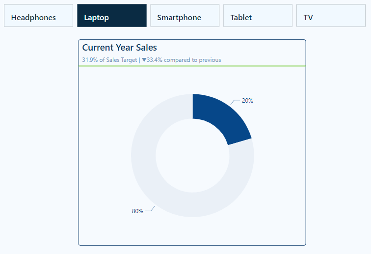
Lastly, we use the empty center of the donut chart to provide additional details to our viewers. Here, we display the total sales value for the selected product and add a dynamic label to clearly show what the sales value represents.
To do this we create another measure to dynamically update based on user selections. The Selected Product measure shows “All Products” when there is no product selection; otherwise, it displays the selected product name, or when there are multiple selections, it displays a list of all the selected products.
Selected Product =
IF (
    ISFILTERED ( Products[Product] ),
    IF (
        HASONEVALUE ( Products[Product] ),
        VALUES ( Products[Product] ),
        CONCATENATEX (
            ALLSELECTED ( Products[Product] ),
            Products[Product],
            ", "
        ) & " Sales"
    ),
    "All Products"
)
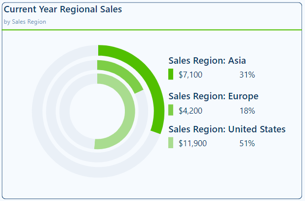
Current Year Regional Sales
The Current Year Regional Sales donut chart compares sales across different sales regions.
We start building this chart with a series of measures. First, a set of measures calculating the current year sales for each region.
Asia Sales CY = CALCULATE([Total Sales CY], Regions[Region]="Asia")
Europe Sales CY = CALCULATE([Total Sales CY], Regions[Region]="Europe")
US Sales CY = CALCULATE([Total Sales CY], Regions[Region]="United States")
Then, we add another set of measures calculating the difference between the total sales and the region-specific sales.
Asia Sales CY Diff = [Total Sales CY] - [Asia Sales CY]
Europe Sales CY Diff = [Total Sales CY] - [Europe Sales CY]
US Sales CY Diff = [Total Sales CY] - [US Sales CY]
Similar to the visual above, we add the region-specific measures to a donut chart and format them to appear as concentric donut charts. This is done by turning off the border and background of the two inner donut charts and resizing them.

Next, we build a customized legend element that not only shows the total sales for each region but also the percentage that each region contributes to the overall sales. The percentage of overall sales is calculated using 3 new measures.
Asia CY % Sales = DIVIDE([Asia Sales CY], [Total Sales CY])
Europe CY % Sales = DIVIDE([Europe Sales CY], [Total Sales CY])
US CY % Sales = DIVIDE([US Sales CY], [Total Sales CY])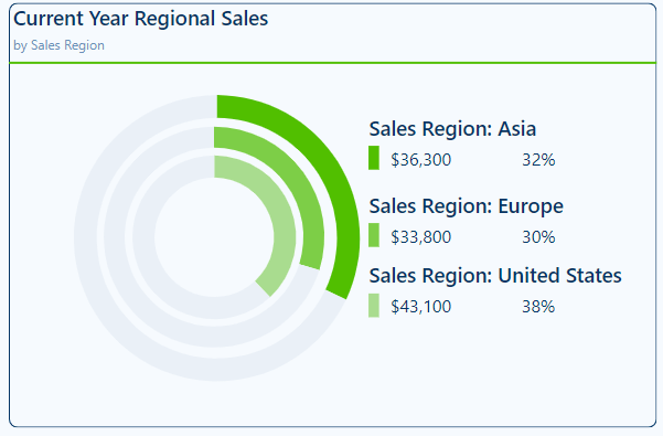
This visual is also dynamic based on the user interaction and selections made on the product slicer.
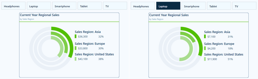
This visual provides our viewers with a quick comparison of regional sales. It clearly shows the sales distribution across our regions, allowing our viewers to identify which regions have the highest or lowest sales.
Wrapping Up
In this part of the series, we explored Pie, Donut, and Treemap charts and how to effectively use and customize these visuals in our Power BI reports. Pie and Donut charts can be helpful tools when displaying proportions but should be used selectively when comparing only a few categories. Treemap charts excel at displaying hierarchical data and provide us with a compact and insightful way to visualize this data.
While these visuals can prove to be just the right fit for a given requirement, they must only be used in the right scenarios, with an emphasis on simplicity and clarity.
In the next part of the series, we will explore Power BI’s Gauge, Card, and KPI visuals. These visuals help us display metrics and provide at-a-glance insights into key data points.
Thank you for reading! Stay curious, and until next time, happy learning.

And, remember, as Albert Einstein once said, “Anyone who has never made a mistake has never tried anything new.” So, don’t be afraid of making mistakes, practice makes perfect. Continuously experiment, explore, and challenge yourself with real-world scenarios.
If this sparked your curiosity, keep that spark alive and check back frequently. Better yet, be sure not to miss a post by subscribing! With each new post comes an opportunity to learn something new.