Design Meets Data: Crafting Interactive Navigations in Power BI


An essential aspect of any multi-page report is an effective and intuitive way to navigate between the various report pages. A well-designed navigational element in our Power BI reports enhances our users’ experience and guides them to the data and visualizations they require.

This post outlines and explores how Power BI native tools and functionalities can be utilized to create a similar navigational experience that was created in the previous post using Figma and Power BI: Design Meets Data: A Guide to Building Interactive Power BI Report Navigation.

Looking for another approach to building report navigation that uses built-in Power BI tools? Visit Part 3 of this Power BI Navigation series.

Streamlined report navigation with built-in tools to achieve functional, maintainable, and engaging navigation in Power BI reports.

For those interested in implementing the navigation element presented in this post, there are 2-, 3-, 4-, and 5-page templates available for download, with more details at the end of the post.

Revisiting Interactive Navigation in Power BI

Welcome back to another Design Meets Data exploration focused on interactive report navigation in Power BI. In the first part, we dove into using Figma to design and develop a user-friendly report interface.

Now, it is time to shift our focus towards leveraging Power BI’s native arsenal of tools, primarily bookmarks, buttons, and tool tips, to achieve similar, if not enhanced, functionalities.

Why go native? Utilizing Power BI’s built-in tools streamlines support and maintenance and provides a reduction in external complexities and dependencies. Plus, staying within a single platform makes it easier to manage and update our reports.

This post will highlight the nuances of Power BI’s navigation capabilities. It will demonstrate how to replicate the interactive navigation from Design Meets Data: A Guide to Building Interactive Power BI Report Navigation using tools available directly within Power BI. These tools will help simplify our report while maintaining an engaging and interactive navigational element.

Let’s get started!


Setting the Stage with Power BI Navigation

Before diving into the details, let’s step back with a quick refresher on the Power BI tools that we can leverage for crafting our report navigation. Power BI is designed to support complex reporting requirements with ease, thanks to features like bookmarks, buttons, and tooltips that can be intricately configured to guide our users through our data seamlessly.

Bookmarks

Bookmarks in Power BI save various states of a report page, allowing users to switch views or data contexts with a single click. We can use bookmarks to allow our users to toggle between different data filters or visual representations without losing context or having to navigate multiple pages.

For our navigational element, bookmarks will be key to creating the collapsing and expanding functionality. To create a bookmark, we get the report page looking just right, then add a bookmark to save the report state in the bookmark pane.

The new bookmark can now act as a restore point, bringing the user back to this specific view whenever it is selected. To keep our bookmarks organized it is best to rename them with a description name, generally including the report page and an indication of what the bookmark is used for (e.g. Page1-NavExpanded).

Buttons

Buttons take interactivity to the next level. We can use buttons to trigger various events, such as bookmarks, and also serve as navigation aids within the report. Buttons within our Power BI reports can be styled and configured to react dynamically to user interactions.

To create a button, we simply add the button object from the Insert ribbon onto the report canvas. Power BI offers a variety of button styles, such as a blank button for custom designs, or predefined icons for common actions like reset, back, or informational buttons.

Each button can be styled to match our report’s theme, including colors, text, and much more. Another key property to configure is the button action. Using this, we can define whether the button should direct our users to a different report page, switch the report context to a different bookmark, or another one of the many options available.

Tooltips

Tooltips in Power BI can provide simple text hints, but when properly utilized, they can provide additional insights or contextual data relevant to specific visuals without cluttering the canvas. This provides detail when required while keeping our reports clean and simple.

Power BI allows us to customize tooltips to show detailed information, including additional visuals. This can turn each tooltip into a tool to provide context or additional layers of data related to a report visual when a user hovers over the element.

By effectively using tooltips we transform user interaction from just viewing to an engaging, exploratory experience. This boosts the usability of our reports and ensures that users can make informed decisions based on the data view provided.


The Navigation Framework

Now that we have explored some details of the elements used to create our navigation, let’s dive into building the navigational framework. We will craft a minimalistic navigation on the left-hand side of our report, with the functionality to expand when requested by user interaction. This approach to our navigation is focused on making the navigation pane both compact and informative, ensuring that it does not overpower the content of the report.

In the Design Meets Data: A Guide to Building Interactive Power BI Report Navigation blog post the navigational element was built using Figma. Although Figma is a powerful and approachable design tool, in this guide, we will explore creating a similar navigation pane using native Power BI tools and elements. We will use Power BI’s shapes, buttons, and bookmarks to construct the framework and functionality.

The Navigation Pane Base Elements

We will start by creating the navigation pane by adding the base elements. In this compact and expandable design, this includes the background of the navigation pane, which will contain the page navigation and menu icons.

Collapsed Navigation Pane

The base of the navigation consists of three main components that we add to our Power BI report to start building our interactive navigational element.

The collapsed navigation pane starts by adding the shape of the pane itself. The color is set to theme color 1, 50% darker of the Power BI theme. Using the theme color will help our navigation remain dynamic when changing Power BI themes.

The next base element is the menu icon, which expands and collapses our navigation pane. The button is configured to slightly darken when hovered over and darken further when pressed. Additionally, when the button is disabled, the icon color is set to the same color as the navigation pane and is used to contrast the current page indicator bar. This configuration is used for all buttons contained within the navigation pane (both the bookmark and page navigation buttons).

The last base element is the current page indicator. This is a lighter-colored (theme color 1, 60% lighter) rectangle tab that clearly indicates what page in the navigation pane is currently being viewed.

Here is the collapsed navigation pane containing the base elements.

Expanded Navigation Pane

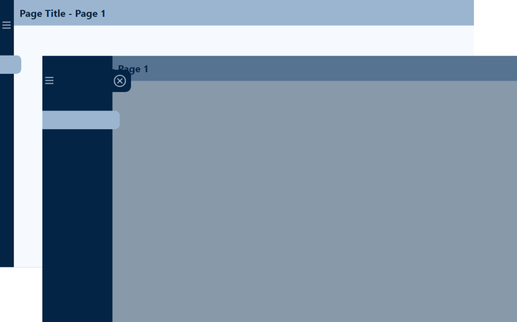
The expanded navigation consists of the same base elements, with the addition of a close icon, and a click shield to prevent the user from interacting with the report visuals when the navigation is expanded.

The additional elements of the expanded menu provide the user with multiple methods to collapse the navigation pane. The close (X) button is added as a flyout from the base navigation pane background, so it is easily identifiable.

When the navigation pane is expanded, we want to prevent users from interacting with the report visuals. To achieve this, we use a partially transparent rectangle to serve as a click shield. If the user clicks anywhere on the report page outside of the navigation pane, the navigation pane will collapse returning the user to the collapsed report view.

Navigation Bookmarks

The last base element required for the interactive navigation is creating the required bookmarks to transition between the collapsed and expanded view. This is done by creating two bookmarks to store each of the required report page views, Page1-Default-NavCollapsed and Page1-NavExpanded.

We can now build on these base elements and bring our navigation to life with Power BI buttons and interactive features.


Navigation Interactive Features

The interactive features in the navigation pane consist of two types of buttons: (1) bookmark buttons and (2) page navigation buttons.

Expanding and Collapsing the Navigation Pane

The previous section added the base elements of the navigation pane which included a menu icon on both the collapsed and expanded navigation panes, and a close button and click shield on the expanded navigation screen.

Building the interactive elements of the navigation starts by assigning actions to each of these bookmark buttons, allowing the user to expand and collapse the navigation pane seamlessly.

The action property for each of these buttons is set to a bookmark type, with the appropriate bookmark selected. For example, for the menu icon button on the collapsed menu, the bookmark selected corresponds to the expanded navigation bookmark. This way, when a user selects this button on the collapsed navigation, it expands, revealing the additional information provided on the expanded navigation pane.

Page Navigation Buttons

The last element to add to the report navigation is the report page navigation buttons.

Each report page button is a blank button configured and formatted to meet the report’s requirements. For this report, each page button contains a circular numbered icon to indicate the report page it navigates to. When the navigation is expanded, an additional text element displays the report page title.

At the end of this post, there are details on obtaining templates that implement this report navigational element. The templates are fully customizable, so they will come with the numbered icons and default page titles, but these can simply be updated to match the aesthetic of any reporting needs.


Wrapping Up: Elevating Your Power BI Reports with Interactive Navigation

As Power BI continues to evolve, integrating more engaging and interactive elements into our reports will become crucial for creating dynamic and user-centric reports. The transition from static to interactive reports empowers our users to explore data in a more meaningful and memorable way. By leveraging bookmarks, buttons, and tooltips, we can transform our reports from a simple presentation of data into engaging, intuitive, and powerful analytical tools.

For those eager to implement the navigational element outlined in this post, there are 2-, 3-, 4-, and 5-page templates available for download. Each template has all the functionality built in, requiring only updating the button icons, if necessary, to better align with your reporting needs.

The template package is available here!

You will get individual template files for a 2-, 3-, 4-, and 5-page report provided in the PBIX, PBIT, and PBIP (12 total files) formats! 


Thank you for reading! Stay curious, and until next time, happy learning.

And, remember, as Albert Einstein once said, “Anyone who has never made a mistake has never tried anything new.” So, don’t be afraid of making mistakes, practice makes perfect. Continuously experiment, explore, and challenge yourself with real-world scenarios.

If this sparked your curiosity, keep that spark alive and check back frequently. Better yet, be sure not to miss a post by subscribing! With each new post comes an opportunity to learn something new.

Dive into DAX: Decoding Data with Power BI Logical Functions


The missing piece to decoding our data and unlocking its full potential is often the strategic application of DAX Logical Functions. These functions are pivotal in dissecting complex datasets, applying business logic, and enabling a nuanced approach to data analysis that goes beyond surface-level insights. Better understanding DAX Logical Functions allows us to create more sophisticated data models that respond with agility to analytical queries, turning abstract numbers into actionable insights.

In this post we will explore this group of functions and how we can leverage them within Power BI. We will dive in and see how we can transform our data analysis from a mere task into an insightful journey, ensuring that every decision is informed, every strategy is data-driven, and every report illuminates a path to action.


The Logical Side of DAX: Unveiling Power BI’s Brain

Diving into the logical side of DAX is where everything begins to become clear. Logical functions are the logical brain behind Power BI’s ability to make decisions. Just like we process information to decide between right and wrong, DAX logical functions sift through our data to determine truth values: true or false.

Functions such as IF, AND, OR, NOT, and TRUE/FALSE, are the building blocks for creating dynamic reports. These functions allow us to set up conditions that our data must meet, enabling a level of interaction and decision-making that is both powerful and nuanced. Whether we are determining if sales targets were hit or filtering data based on specific criteria, logical functions are our go-to tools for making sense of the numbers.

For details on these functions and many others visit the DAX Function Reference documentation.

Learn more about: DAX Logical Functions

The logical functions in DAX can go far beyond the basics. The real power happens when we start combining these functions to reflect complex business logic. Each function plays its role and when used in combination correctly we can implement complex logic scenarios.

For those eager to start experimenting there is a Power BI report pre-loaded with the same data used in this post ready for you! So don’t just read, follow along and get hands-on with DAX in Power BI. Get a copy of the sample data report here:

This dynamic repository is the perfect place to enhance your learning journey.


Understanding DAX Logical Functions: A Beginner’s Guide

When starting our journey with DAX logical functions we will begin to understand the unique role of each function within our DAX expressions. Among these functions, the IF function stands out as the decision-making cornerstone.

The IF function tests a condition, returning one result if the condition is TRUE, and another if FALSE. Here is its syntax.

IF(logical_test, value_if_true, value_if_false)

The logical_test parameter is any value or expression that can be evaluated to TRUE or FALSE, and then the value_if_true is the value that is returned if logical_test is TRUE, and the value_if_false is optional and is the value returned when logical_test is FALSE. When value_if_false is omitted, BLANK is returned when the logical_test is FALSE.

Let’s say we want to identify which sales have an amount that exceeds $5,000. To do this we can add a new calculated column to our Sales table with the following expression.

Sales Target Categorization = 
IF(
  Sales[Amount] > 5000, 
  "Above Target", 
  "Below Target"
)

This expression will evaluate each sale in our Sales table, labeling each sale as either “Above Target” or “Below Target” based on the Sales[Amount].

The beauty of starting our journey with IF lies in its simplicity and versatility. While we continue to explore logical functions, it won’t be long before we encounter TRUE/FALSE.

As we saw with the IF function these values help guide our DAX expressions, they are also their own DAX function. These two functions are the DAX way of saying yes (TRUE) or no (FALSE), often used within other logical functions or conditions to express a clear binary choice.

These functions are as straightforward as they sound and do not require any parameters. When used with other functions or conditional expressions we typically use these to explicitly return TRUE or FALSE values.

For example, we can create another calculated column to check if a sale is a high value sale with an amount greater than $9,000.

High Value Sale = 
IF(
  Sales[Amount] > 9000, 
  TRUE, 
  FALSE
)

This simple expression checks if the sales amount exceeds $9,000, marking each record as TRUE if so, or FALSE otherwise.

Together IF and TRUE/FALSE form the foundation of logical expressions in DAX, setting the stage for more complex decision-making analysis. Think of these functions as essential for our logical analysis, but just the beginning of what is possible.


The Gateway to DAX Logic: Exploring IF with AND, OR, and NOT

The IF function is much more than just making simple true or false distinctions; it helps us unlock the nuanced layers of our data, guiding us through the paths our analysis can take. By effectively leveraging this function we can craft detailed narratives from our datasets.

We are tasked with setting sales targets for each region. The goal is to base these targets on a percent change seen in the previous year. Depending on whether a region experienced a growth or decline, the sales target for the current year is set accordingly.

Region Specific Sales Target = 
IF(
    HASONEVALUE(Regions[Region]),
    IF(
        [Percent Change(CY-1/CY-2)] < 0, 
        [Total Sales (CY-1)]*1.1, 
        [Total Sales (CY-1)]*1.2
    ),
    BLANK()
)

In this measure we make use of three other measures within our model. We calculate the total sales for the previous year (Total Sales (CY-1)), and the year before that (Total Sales (CY-2)). We then determine the percentage change between these two values.

If there is a decline (negative percent change), we set the current year’s sales target to be 10% higher than the previous year’s sales, indicating a more conservative goal. Conversely, if there was growth (positive percent change), we set the current year target 20% higher to keep the momentum going.

As we dive deeper, combining IF with functions like AND, OR, and NOT we begin to see the true flexibility of these functions in DAX. These logical operators allow us to construct more intricate conditions, tailoring our analysis to very specific scenarios.

The operator functions are used to combine multiple conditions:

  • AND returns TRUE if all conditions are true
  • OR returns TRUE if any condition is true
  • NOT returns TRUE if the condition is false

Let’s craft a measure to determine which employees are eligible for a quarterly bonus. The criterion for eligibility is twofold: the employee must have made at least one sale in the current quarter, and their average sale amount during this period must exceed the overall average sale amount.

To implement this, we first need to calculate the average sales and compare each employee’s average sale against this benchmark. Additionally, we check if the employee has sales recorded in the current quarter to qualify for the bonus.

Employee Bonus Eligibility = 
VAR CurrentQuarterStart = DATE(YEAR(TODAY()), QUARTER(TODAY()) * 3 - 2, 1)
VAR CurrentQuarterEnd = EOMONTH(DATE(YEAR(TODAY()), QUARTER(TODAY()) * 3, 1), 0)
VAR OverallAverageSale = CALCULATE(AVERAGE(Sales[Amount]), ALL(Sales))
VAR EmployeeAverageSale = CALCULATE(AVERAGE(Sales[Amount]), FILTER(Sales, Sales[SalesDate] >= CurrentQuarterStart && Sales[SalesDate] = CurrentQuarterStart && Sales[SalesDate]  0

RETURN
IF(
    AND(HasSalesCurrentQuarter, EmployeeAverageSale > OverallAverageSale),
    "Eligible for Bonus",
    "Not Eligible for Bonus"
)

In this measure we define the start and end dates of the current quarter, then we calculate the overall average sale across all data for comparison. We then determine each employee’s average sale amount and check if the employee has made any sales in the current quarter to qualify for evaluation.

If an employee has active sales and their average sale amount during the period is above the overall average, they are deemed “Eligible for Bonus”. Otherwise, they are “Not Eligible for Bonus”.

This example begins to explore how we can use IF in conjunction with AND to streamline business logic into actionable insights. These logical functions provide a robust framework for asking detailed questions about our data and receiving precise answers, allowing us to uncover the insights hidden within the numbers.


Beyond the Basics: Advanced Logical Functions in DAX

As we venture beyond the foundational logical functions we step into a world where DAX’s versatility shines, especially when dealing with complex data models in Power BI. More advanced logical functions such as SWITCH and COALESCE bring a level of clarity and efficiency that is hard to match with just basic IF statements.

SWITCH Function: Simplifying Complex Logic

The SWITCH function is a more powerful version of the IF function and is ideal for scenarios where we need to compare a single expression against multiple potential values and return one of multiple possible result expressions. This function helps us provide clarity by avoiding multiple nested IF statements. Here is its syntax.

SWITCH(expression, value, result[, value, result]...[, else])

The expression parameter is a DAX expression that returns a single scalar value and is evaluated multiple times depending on the context. The value parameter is a constant value that is matched with the results of expression, the result is any scalar expression to be evaluated if the result of expression matches the corresponding value. Finally, the else parameter is an expression to be evaluated if the result of expression does not match any value arguments.

Let’s explore. We have a scenario where we want to apply different discount rates to products based on their categories (Smartphone, Laptop, Tablet). We could achieve this by using the following expression for a new calculated column, which uses nested IFs.

Product Discount Rate (IF) = 
IF(
    Products[Product]="Smartphone", 0.10,
    IF(Products[Product]="Laptop", 0.15,
        IF(Products[Product]="Tablet", 0.20,
            0.05
        )
    )
)

Although this would achieve our goal, the use of nested if statements can make the logic of the calculated column hard to read, understand, and most importantly hard to troubleshoot.

Now, let’s see how we can improve the readability and clarity by implementing SWITCH to replace the nested IF statements.

Product Discount Rate = 
SWITCH(
    Products[Product],
    "Smartphone", 0.10,
    "Laptop", 0.15,
    "Tablet", 0.20,
    0.05
)

The expression simplifies the mapping of each Product to its corresponding discount rate and provides a default rate for categories that are not explicitly listed.

COALESCE Function: Handling Blank or Null Values

The COALESCE function offers a straightforward way to deal with BLANK values within our data, returning the first non-blank value in a list of expressions. If all expressions evaluate to BLANK, then a BLANK value is returned. Its syntax is also straightforward.

COALESCE(expression, expression[, expression]...)

Here, expression can be any DAX expression that returns a scalar value. These expressions are evaluated in the order they are passed to the COALESCE function.

When reporting on our sales data, encountering blanks can sometimes communicate the wrong message. Using COALESCE we can address this by providing a more informative value when there are no associated sales.

Product Sales = COALESCE([Total Sales], "No Sales")

With this new measure if our Total Sales measure returns a blank, for example due to filters applied in the report, COALESCE ensures this is communicated with a value of “No Sales”. This approach can be beneficial for maintaining meaningful communication in our reports. It ensures that our viewers understand the lack of sales being reported, rather than interpreting a blank space as missing or erroneous data.

These logical functions enrich our DAX toolkit, enabling more elegant solutions to complex problems. By efficiently managing multiple conditions and safeguarding against potential errors, SWITCH and COALESCE not only optimize our Power BI models but also enhance our ability to extract meaningful insights from our data.

With these functions, our journey into DAX’s logical capabilities becomes even more exciting, revealing the depth and breadth of analysis we can achieve. Let’s continue to unlock the potential within our data, leveraging these tools to craft insightful, dynamic reports.


Logical Comparisons and Conditions: Crafting Complex DAX Logic

Delving deeper into DAX, we encounter scenarios that demand a blend of logical comparisons and conditions. This complexity arises from weaving together multiple criteria to craft intricate logic that precisely targets our analytical goals.

We touched on logical operators briefly in a previous section, the AND, OR, and NOT functions are crucial for building complex logical structures. Let’s continue to dive deeper into these with some more hands-on and practical examples.

Multi-Condition Sales Analysis

We want to identify and count the number Sales transactions that meet specific criteria: sales above a threshold and within a particular region. To achieve this, we create a new measure using the AND operator to count the rows in our sales table that meet our criteria.

High Value Sales in US (Count) = 
COUNTROWS(
    FILTER(
        Sales,
        AND(
            Sales[Amount] > 5500,
            RELATED(Regions[Region]) = "United States"
        )
    )
)

This measure filters our Sales table to sales that have an amount greater than our threshold of $5,500 and have a sales region of United States.

Excluding Specific Conditions

We need to calculate total year-to-date sales while excluding sales from a particular region or below a certain amount. We can leverage the NOT function to achieve this.

Sales Excluding Asia and Low Values = 
CALCULATE(
    SUM(Sales[Amount]),
    AND(
        NOT(Sales[RegionID] = 3), // RegionID=3 (Asia)
        Sales[Amount] > 5500
    ),
    Sales[IsCurrentYear]=TRUE()
)

This measure calculates the sum of the sales amount that are not within our Asia sales region and are above $5,500. Using NOT we exclude sales from the Asia region and we us the AND function to also impose the minimum sales amount threshold.

Special Incentive Qualifying Sales

Our goal is to identify sales transactions eligible for a special incentive based on multiple criteria: sales amount, region, employee involvement, and a temporal aspect of the sales data. Here is how we can achieve this.

Special Incentive Qualifying Sales = 
CALCULATE(
    SUM(Sales[Amount]),
    OR(
        Sales[Amount] > 7500,
        Sales[RegionID] = 2
    ),
    NOT(
        Sales[EmployeeID] = 4
    ),
    Sales[IsCurrentYear] = TRUE()
)

The OR function is used to include sales transactions that either exceed $7,500 or are made in Europe (RegionID = 2) and the NOT function excludes transaction made by an employee (EmployeeID = 4), who is a manager and exempt from the incentive program. The final condition is that the sale occurred in the current year.

The new measure combines logical tests to filter our sales data, identifying the specific transactions that qualify for a special incentive under detailed conditions.

By leveraging DAX’s logical functions to construct complex conditional logic, we can precisely target specific segments of our data, uncover nuanced insights, and tailor our analysis to meet specific business needs. These examples showcase just the beginning of what is possible when we combine logical functions in creative ways, highlighting DAX’s robustness and flexibly in tackling intricate data challenges.


Wrapping Up: From Logic to Action

Our journey through the world of DAX logical functions underscores their transformative power within our data analysis. By harnessing IF, SWITCH, AND, OR, and more, we’ve seen how data can be sculpted into actionable insights, guiding strategic decisions with precision. To explore other DAX Logical Functions or get more details visit the DAX Function Reference.

Learn more about: DAX Logical Functions

Logical reasoning in data analysis is fundamental. It allows us to uncover hidden patterns and respond to business needs effectively, demonstrating that the true value of data lies in its interpretation and application. DAX logical functions are the keys to unlocking this potential, offering clarity and direction in our sea of numbers.

As we continue to delve deeper into DAX and Power BI, let the insights derived from logical functions inspire action and drive decision-making. To explore other functions groups that elevate our data analysis check out the Dive into DAX series, with each post comes the opportunity to enhance your data analytics and Power BI reports.

Explore the intricate landscape of DAX in Power BI, revealing the potential to enhance your data analytics with every post. 


Thank you for reading! Stay curious, and until next time, happy learning.

And, remember, as Albert Einstein once said, “Anyone who has never made a mistake has never tried anything new.” So, don’t be afraid of making mistakes, practice makes perfect. Continuously experiment and explore new DAX functions, and challenge yourself with real-world data scenarios.

If this sparked your curiosity, keep that spark alive and check back frequently. Better yet, be sure not to miss a post by subscribing! With each new post comes an opportunity to learn something new.

DAX Filter Functions: Navigating the Data Maze with Ease


In the intricate world of Power BI, the ability to skillfully navigate through complex data models is not just a skill, but an art form. This is where DAX Filter Functions come into play, serving as our compass in the often-overwhelming maze of data analysis. These functions give us the power to sift through layers of data with intent and precision, uncovering insights that are pivotal to informed decision-making.

Our journey through data analysis should not be a daunting task. With the right tools and know-how, it can become an adventure in discovering hidden patterns and valuable insights. DAX Filter Functions are the keys to unlocking this information, allowing us to filter, dissect, and examine our data in ways we never thought possible.

Now, let’s embark on a journey to master these powerful functions. Transform our approach to data analysis in Power BI, making it more intuitive, efficient, and insightful. Let DAX Filter Functions guide us through the data maze with ease, leading us to clarity and success in our data analysis endeavors. The path to elevating our Power BI skills starts here, and it starts with mastering DAX Filter Functions.

For those of you eager to start experimenting there is a Power BI report-preloaded with the same data used in this post read for you. So don’t just read, follow along and get hands-on with DAX in Power BI. Get a copy of the sample data file here:

This dynamic repository is the perfect place to enhance your learning journey.


What are DAX Filter Functions

DAX filter functions are a set of functions in Power BI that allow us to filter data based on specific conditions. These functions help in reducing the number of rows in a table and allows us to focus on specific data for calculations and analysis. By applying well defined filters, we can extract meaningful insights from large datasets and make informed business decisions. Get all the details on DAX Filter Functions here.

Learn more about: Filter functions

In our Power BI report, we can use filter functions in conjunction with other DAX functions that require a table as an argument. By embedding these functions, we can filter data dynamically to ensure our analysis and calculation are using exactly the right data. Let’s dive into some of the commonly used DAX filter functions and explore their syntax and usage.


The ALL Function: Unleashing the Potential of All Our Data

At its core, the ALL function is a powerhouse of simplicity and efficiency. It essentially removes all filters from a column or table, allowing us to view our data in its most unaltered form. This function is our go to tool when we need to clear all filters to create calculation using all the rows in a table The syntax is straightforward:

ALL([table | column[, column[, column[,...]]]])

The arguments to the ALL function must either reference a base table or a base column of the data model, we cannot use table or column expressions with the ALL function. This function serves as a intermediate function that we can use to change the set of results over which a calculation is performed.

ALL can be used in a variety of ways when referencing base tables or columns. Using ALL() will remove filters everywhere and can only be used to clear filters but does not return a table. When referencing a table, ALL(<table>), the function removes all the filters from the specified table and returns all the values in the table. Similarly, when referencing columns, ALL([, [, ...]]), the function removes all filters from the specified column(s) in the table, while all other filters on other column in the table still apply. When referencing columns, all the column argument must come from the same table.

While, we can use ALL to remove all context filters from specified columns, there is another function that can be helpful. ALLEXCEPT is a DAX function that removes all context filters in the table except filters that have been applied to the specified columns. For more details check out the Microsoft documentation on ALLEXCEPT.

Learn more about: ALLEXCEPT

Practical Examples: Navigating Data with the ALL Function

Considering the dataset in our sample report, suppose we want to analyze the overall sales performance, irrespective of any specific regions or dates. Using the following formula, we can provide the total sales amount across all regions and times by removing any existing filters on the Sales table.

All Sales = 
SUMX(
   ALL(Sales), 
   Sales[Amount]
)

In the above example we can see the card visual on the bottom left is the default sum aggregation of the Amount column in our sales table. Specifically, with the slicers on the report, this card shows the total sales within the United States region during the period between 1/1/2023 and 3/31/2023. We can use the ALL function to display to total sales amount across all regions and irrespective of time, shown on the card visual on the right.

This functionality is particularly useful when making comparative analyses. For instance, we could use this to determine a region’s contribution to total sales. We can compare the sales in a specific region (with filters applied) to the overall sales calculated using ALL. This comparison offers valuable insights into the performance of different segments relative to the total context.


ALLSELECTED Decoded: Interactive Reporting’s Best Friend

The ALLSELECTED function in DAX takes the capabilities of ALL a step further. It is particularly useful in interactive reports where our users apply filters. This function respects the filters applied by our report users but disregards any filter context imposed by report objects like visuals or calculations. The syntax is:

ALLSELECTED([tableName | columnName[, columnName[, columnName[,…]]]] )

Similar to ALL the tableName and columnName parameters are optional and reference an existing table or column, an expression cannot be used. When we provide ALLSELECTED a single argument it can either be tableName or columnName, and when we provide the function more than one argument, they must be columns from the same table.

ALLSELECTED differs from ALL because it retains all filters explicitly set within the query, and it retains all context filters other than row and column filters.

Practical Examples: Exploring ALLSELECTED and How it Differs From ALL

At first glance it may seem as if ALL and ALLSELECTED perform the same task. Although, these two functions are similar there is an important difference between them. ALLSELECTED will ignore filters applied by report visuals, while ALL will ignore any filters applied within the report. Let’s explore this difference with an example.

We will use three measures to explore ALLSELECTED. First a measure that simply calculates the sum of our Sales Amount, here is its definition.

Total Sales = SUM(Sales[Amount])

Second a measure using the function explored in the previous section ALL.

Sales ALL = CALCULATE(
    SUM(Sales[Amount]),
    ALL(Sales)
)

Lastly, a measure that uses ALLSELECTED.

Sales ALLSELECTED = 
CALCULATE(
    SUM(Sales[Amount]),
    ALLSELECTED(Sales)
)

After creating the measures, we can add a table visual including the Product field and these three measures. When the report has no filters due to interacting with the slicers on the report, we can see that the Total Sales measure gets filtered by the Product column and shows the total sales for each product. However, the other two measure show the overall total sales.

The inclusion of the Product column in the table visual is filtering the values and impacting the calculation of the Total Sales measure, while the other two measure are using all of the sales records in their calculation.

Next let’s use the Region and Date slicers to explore the differences between ALL and ALLSELECTED. As expected, all the additional filtering due to the slicer selections continues to impact our Total Sales measure.

Additionally, we see the ALLSELECTED measure gets filtered based on the external slicer selections but continues to not be impacted by the internal filtering of the table visual. This differs from our measure that uses the ALL function, which continues to show the grand total sales value. This is because the ALL function ignores any filter implicit from the visual or explicit from external slicers.

The difference between ALL and ALLSELECTED boils down to ALL will ignore any filter applied, while ALLSELECTED will ignore just the filter applied by the visual.

The necessity of ALLSELECTED is its ability to respect user’s interactions and filtering choices on slicers or other interactive elements. Unlike ALL, which disregards all filters, ALLSELECTED maintains the interactive nature or our reports, ensuring that the calculations dynamically adapt to user inputs.

So, what is a use case for ALLSELECTED? A common use is calculating percentages, based on a total value that is dependent on user interaction with report slicers. Check out this post, on how this function can be used along with ISINSCOPE to calculate context aware insights.

Elevate Your Power BI Report with Context-Aware Insights


CALCULATE: The Engine for Transforming Data Dynamically

CALCULATE is one of the most versatile and powerful functions in DAX, acting as a cornerstone for many complex data operations in Power BI. It allows us to manipulate the filter context of a calculation, letting us perform dynamic and complex calculations with ease. CALCULATE follows a simple structure.

CALCULATE(expression[, filter1[, filter2[, …]]])

The expression parameter is the calculation we want to perform, and the filter parameters are optional boolean expressions or table expression that define our filters or filter modifier functions. Boolean filter expressions are expressions that evaluate to true or false, and when used with CALCULATE there are certain rules that must be followed, see the link below for details. Table filter expressions apply to a table, and we can use the FILTER function to apply more complex filtering conditions, such as those that cannot be defined by using a boolean filter expression. Finally, filter modifier functions provide us even more control when modifying the filter context within the CALCULATE function. Filter modifier functions include functions such as REMOVEFILTERS, KEEPFILTERS, and the ALL function discussed in the previous section.

Find all the required details in the documentation.

Learn more about: CALCULATE

Practical Examples: Using CALCULATE for Dynamic Data Analysis

Let’s say that for our report we are required to calculate the total sales in the United States region. We can use CALCULATE and this expression to meet this requirement.

United States Sales = 
CALCULATE(
   SUM(Sales[Amount]), 
   Regions[Region]="United States"
)

We can continue to build on the previous example to further examine sales in the United States. For this example, we will compare the average sales of smartphones in the United States against the benchmark of average sales of smartphones across all regions.

US Smartphone Sales vs. Average Smartphone Sales =
    CALCULATE(
        AVERAGE(Sales[Amount]),
        Products[Product] = "Smartphone",
        Regions[Region] = "United States"
    )
    - AVERAGEX(
        FILTER(
            Sales,
            RELATED(Products[Product]) = "Smartphone"
        ),
        Sales[Amount]
)

These two examples just begin to scratch the surface of what is possible when we utilize the CALCULATE function. For more examples and more details on CALCULATE check out this post that provides a deep dive into the CALCULATE function.

Demystifying CALCULATE: An exploration of advanced data manipulation. 

CALCULATE proves indispensable for redefining the filter context impacting our calculations. It empowers us to perform targeted analysis that goes beyond the standard filter constraints of a report, making it an essential tool in our DAX toolbox.


Mastering FILTER: The Art of Precision in Data Selection

The FILTER function in DAX is a precision tool for refining data selection within Power BI. It allows us to apply specific conditions to a table or column, creating a subset of data that meets the criteria. The FILTER function returns a table that represents a subset of another table or expression, and the syntax is as follows.

FILTER(table, filter)

The table argument is the table, or an expression that results in a table, that we want to apply the filter to. The filter argument is a boolean expression that should be evaluated for each row of the table.

FILTER is used to limit the number of rows in a table allowing for us to create specific and precise calculations. When we use the FILTER function we embed it within other functions, we typically do not use it independently.

When developing our Power BI reports a common requirement is to develop DAX expressions that need to be evaluated within a modified filter context. As we saw in the previous section CALCULATE is a helpful function to modify the filter context, and accepts filter arguments as either boolean expressions, table expression or filter modification functions. Meaning CALCULATE, will accept the table returned by FILTER as one of its filtering parameters, however it is generally best practice to avoid using the FILTER function as a filter argument when a boolean expression can be used. The FILTER function should be used when the filter criteria cannot be achieved with a boolean expression. Here is an article that details this recommended best practice.

Best practices for using the FILTER function as a filter argument.

For example, we have two measures below that calculate the total sales amount for the United States. Both of these measures correctly filter our data and calculate the same value for the total sales. When possible, the best practice is to use the expression on the left which passes the filter arguments to CALCULATE as a boolean expression. This is because when working with Import model tables that are store in-memory column stores, they are explicitly optimized to filter column in this way.

Practical Examples: FILTER Functions Illustrated

Let’s now see how FILTER can help us build on our analysis of US Smartphone Sales. In the previous section we created a US Smartphone Sales vs Average Smartphone Sales measure to visualize US sales against a benchmark. Now we are interested in the total sales amount for each quarter that average US smartphones sales is below the benchmark. FILTER can help us do this with the following expression.

United States Sales FILTER = 
   CALCULATE(
      SUM(Sales[Amount]), 
      FILTER(
         VALUES(DateTable[YearQuarter]), 
         [US Smartphone Sales vs. Average Smartphone Sales] &lt; 0
      )
   )

FILTER is particularly useful when we require a detailed and specific data subset. It is a function that brings granular control to our data analysis, allowing for a deeper and more focused exploration of our data.


Dynamic Table Creation with CALCULATETABLE

The CALCULATETABLE function in DAX is a powerful tool for creating dynamic tables based on specific conditions. This function performs provides us the same functionality that CALCULATE provides, however rather than returning a singular scalar value CALCULATETABLE returns a table. Here is the function’s syntax:

CALCULATETABLE(expression[, filter1[, filter2[, …]]])

This may look familiar, CALCULATETABLE has the same structure as CALCULATE for details on the expression and filter arguments check out the previous section focused on the CALCULATE function.

Practical Examples: Apply CALCULATETABLE

Let’s say we want to calculate the total sales for the current year so we can readily visualize the current year’s sale broken down by product, region and employee. CALCULATETABLE can help us achieve this with the following expression.

Current Year Total Sales = 
SUMX(
   CALCULATETABLE(
      Sales, 
      YEAR(Sales[SalesDate]) = YEAR(TODAY())
   ), 
   Sales[Amount]
)

CALCULATETABLE proves to be invaluable when we need to work with a subset of data based on dynamic conditions. It’s flexibility to reshape our data on the fly makes it an essential function for nuanced and specific data explorations in Power BI.


Resetting the Scene with REMOVEFILTERS

The REMOVEFILTERS function in DAX is crucial for when we need to reset or remove specific filters applied to our data. It allows for recalibration of the filter context, either entirely or partially. The syntax for this function is:

REMOVEFILTERS([table | column[, column[, column[,…]]]])

Looking at the structure of REMOVEFILTERS, we can see it is similar to that of ALL and ALLSELECTED. Although these functions are similar it is important to differentiate them. While ALL removes all filters from a column or table and ALLSELECTED respects user-applied filter but ignores other filter contexts, REMOVEFILTERS specifically targets and removes filters from the specified columns or tables, offering us more control and precision.

Practical Examples: Implementing REMOVEFILTERS

Let’s start by adding a new measure to our previous table visual where we explored the difference between ALL and ALLSELECTED to highlight the difference between these functions.

We will create a new measure and add it to the table visual, the new measure is:

Sales REMOVEFILTER Region = 
CALCULATE(
   SUM(Sales[Amount]), 
   REMOVEFILTERS(Regions[Region])
)

This expression will calculate the total sales disregarding any Region filter that might be in place.

Here we can see this new Sales REMOVEFILTER Region measure shows the total sales respecting the row context of Product on the table visual and the selected dates on the date slicer, however, removes the Region filter that would apply due to the Region slicer.

Let’s take a look at how we can apply and leverage the differences between these functions. We can use our Total Sales and the other three measures to calculate various percentages to provide additional insights.

REMOVEFILTERS offers a tailored approach to filter removal, differing from ALL which disregards all filters unconditionally, and ALLSELECTED which adapts to user selections. This makes REMOVEFILTERS an essential function for creating more nuanced and specific measures in our Power BI reports.


LOOKUPVALUE: Bridging Tables in Analysis

The LOOKUPVALUE function in DAX is a powerful feature for cross-referencing data between tables. It allows us to find a value in a table based on matching a value in another table or column.

LOOKUPVALUE (
    result_columnName,
    search_columnName,
    search_value
    [, search2_columnName, search2_value]…
    [, alternateResult]
)

Here result_columnName is the name of an existing column that contains the value we want to be returned by the function; it cannot be an expression. The search_columnName argument is the name of an existing column and can be in the same table as the result_columnName or in a related table, the search_value is the value to search for within the search_columnName. Finally, the alternativeResult is an optional argument that will be returned when the context for result_columnName has been filter down to zero or more than one district value, when not specified LOOKUPVALUE will return BLANK.

LOOKUPVALUE is essential for scenarios where data relationships are not directly defined through relationships in the data model. If there is a relationship between the table that contains the result column and tables that contain the search column, typically using the RELATED function rather than LOOKUPVALUE is more efficient.

Practical Examples: LOOKUPVALUES Explored

Let’s use LOOKUPVALUE to connect sales data with the respective sales managers. We need to identify the manager for each sale in our Sales table for our report. We can use a formula that first finds the manager’s ID related to each sale. For details on how we can user Parent and Child Functions to work with hierarchical data check out the Parent and Child Functions: Managing Hierarchical Data section of this post.

Unlock the Full Potential of Your Data with DAX: From Basic Aggregations to Advanced Time Intelligence

In the example in the post above we use PATH and PATHITMEREVERSE to navigate the organizational hierarchy to identify the manager’s ID of each employee. Then utilizing REALTED and LOOKUPVALUE we can add a new calculated column to our Sales table listing the Sales Manager for each sale. We can use the following formula that first finds the manager’s ID related to each sale and then fetches the manager’s name using the LOOKUPVALUE function.

Sales Manager Name = 
VAR ManagerID = RELATED(Employee[ManagerID])

RETURN
LOOKUPVALUE(Employee[EmployeeName], Employee[EmployeeID], ManagerID)

In this example, the RELATED function retrieves the ManagerID for each sale from the Employees table. Then, LOOKUPVALUE is used to find the corresponding EmployeeName (the manager’s name) in the same table based on the ManagerID. This approach is particulariy beneficial in scenarios where understanding hierarchical relationships or indirect associations between data points is crucial.

By using LOOKUPVALUE in this manner, we add significant value to our reports, offering insights into the managerial oversight of sales activities, which can be pivotal for performance analysis and strategic planning.


Mastering DAX Filter Functions for Advanced Analysis

Now that we have finished our exploration of DAX Filter Functions in Power BI, it is clear that these tools are not just functions, they are the building blocks for sophisticated data analysis. From the comprehensive clearing of contexts with ALL to dynamic and context-sensitive capabilities of CALCULATE and FILTER, each function offers a unique approach to data manipulation and analysis.

Understanding and applying functions like ALLSELECTED, REMOVEFILTERS and LOOKUPVALUE enable us to create reports that are not only insightful but also interactive and responsive to user inputs. They allow use to navigate through complex data relationships with ease, bringing clarity and depth to our analyses.

As we continue our journey in data analytics, remember that mastering these functions can significantly enhance our ability to derive meaningful insights from our data. Each function has its place and purpose, and knowing when and how to use them will set us apart as proficient Power BI analyst.

Embrace these functions as we delve deeper into our data and watch as they transform our approach to business intelligence and data storytelling. Happy analyzing!


Thank you for reading! Stay curious, and until next time, happy learning.

And, remember, as Albert Einstein once said, “Anyone who has never made a mistake has never tried anything new.” So, don’t be afraid of making mistakes, practice makes perfect. Continuously experiment and explore new DAX functions, and challenge yourself with real-world data scenarios.

If this sparked your curiosity, keep that spark alive and check back frequently. Better yet, be sure not to miss a post by subscribing! With each new post comes an opportunity to learn something new.