Slicers are some of the most commonly used elements in Power BI, yet they often receive less attention than they deserve. They are frequently added to a report, filled with data, and then left for users to navigate on their own.

Users understand their selections, but often lack additional context to inform their decisions. Choosing a category or product line is straightforward, yet the impact of that choice remains unclear until after the selection is made.

We can design our slicers to do more. By displaying preview counts, averages, or percentages, they give users a better understanding of scale and significance before making decisions. This results in smoother exploration and more confident choices, allowing slicers to actively guide analysis rather than merely filtering data.

A sample report is available at the end of this post. Visit the sample report below to explore the examples in action!

From Static Slicers to Interactive Decision Aids – Sample Power BI Report

Building the First Dynamic Slicer with Count of Sales

Let’s begin with a straightforward example of this method, where we display counts next to each slicer value. Instead of selecting an option and waiting for a visual update, or using limited canvas space to show a simple count, the user can see the amount of data associated with each choice directly within the slicer.

Thanks to Davide Bacci (GitHub – PBI-David/PBI-Core-Visuals-SVG-HTML) for the idea and the DAX measures that got us started.

We are developing a sales region slicer. Typically, a user would only see the list of regions. By adding a measure that calculates the number of related sales records for each option, we can transform that list into a preview of the selection’s impacts.

The pattern utilizes the Power BI list slicer, coupled with an SVG measure used for its image property based on the button selection state (default, hover, pressed, selected).

Step #1 – Base Metric

The base metric is the measure displayed to the right of the sales region name. For our first example, this is a simple count of our sales records.

Sales Count = COUNTROWS(Sales)

Step #2 – Centralized Styling

We style the SVG with CSS, allowing us to set colors, fonts, and other aesthetics for the different button states (default, hover, selected, etc.).

SVG Slicer Styling = "
<style>
.slicerTextDefault {
    font:9pt Segoe UI Regular;
    fill:#9FC2D9;
    text-anchor: end;
    alignment-baseline: middle
    }

.slicerTextHover {
    font:9pt Segoe UI Regular;
    fill:#FFFFFF;
    text-anchor: end;
    alignment-baseline: middle
    }

.slicerTextPressed {
    font:9pt Segoe UI Regular;
    fill:#FFFFFF;
    text-anchor: end;
    alignment-baseline: middle
    }

.slicerTextSelected {
    font:9pt Segoe UI Regular;
    fill:#073450;
    text-anchor: end;
    alignment-baseline: middle
    }
</style>
"
    

Step #3 – SVG Measure

Next, we create the SVG measure for each state we are targeting.

SVG Slicer Default =
"data:image/svg+xml;utf8,
<svg xmlns='http://www.w3.org/2000/svg' viewBox='0 0 100% 100%'>" & [SVG Slicer Styling] & "
<rect x='0' y='0' width='100%' height='100%' fill='transparent'></rect>
<text x='100%' y='55%' class='slicerTextDefault'>(" & FORMAT([Sales Count], "#,#") & ")</text>
</svg>"

SVG Slicer Hover =
"data:image/svg+xml;utf8,
<svg xmlns='http://www.w3.org/2000/svg' viewBox='0 0 100% 100%'>" & [SVG Slicer Styling] & "
<rect x='0' y='0' width='100%' height='100%' fill='transparent'></rect>
<text x='100%' y='55%' class='slicerTextHover'>(" & FORMAT([Sales Count], "#,#") & ")</text>
</svg>"

SVG Slicer Pressed =
"data:image/svg+xml;utf8,
<svg xmlns='http://www.w3.org/2000/svg' viewBox='0 0 100% 100%'>" & [SVG Slicer Styling] & "
<rect x='0' y='0' width='100%' height='100%' fill='transparent'></rect>
<text x='100%' y='55%' class='slicerTextPressed'>(" & FORMAT([Sales Count], "#,#") & ")</text>
</svg>"

SVG Slicer Selected =
"data:image/svg+xml;utf8,
<svg xmlns='http://www.w3.org/2000/svg' viewBox='0 0 100% 100%'>" & [SVG Slicer Styling] & "
<rect x='0' y='0' width='100%' height='100%' fill='transparent'></rect>
<text x='100%' y='55%' class='slicerTextSelected'>(" & FORMAT([Sales Count], "#,#") & ")</text>
</svg>"

Step #4 – Build the List Slicer

We add the List Slicer visual to our report and set the Slicer settings, Layout, Callout values, and Buttons properties to meet our reporting needs and styling requirements.

Then we move to the Images property to take our slicer from basic to a decision aid. Using the State dropdown menu, we set the following measures for the field property.

• Default: SVG Slicer Default
• Hover: SVG Slicer Hover
• Pressed: SVG Slicer Pressed
• Selected: SVG Slicer Selected

The result is a dynamic slicer that provides context before a choice is made. This enhances the data exploration experience, allowing for informed and confident selections.

From Totals to Insight: Rich Previews on Your Slicer

Displaying record counts is a good starting point, but we can expand on this idea. Instead of showing just totals, we can surface insights that make the slicer a guide rather than just a filter.

Make it Reusable & Maintainable

Before jumping into examples, let’s first make our SVG Slicer measures easier to reuse and update. We will replace the explicit measure used for display (e.g. [Number of Sales]) with a single new measure, [SVG Slicer Display].

SVG Slicer Default =
"data:image/svg+xml;utf8,
<svg xmlns='http://www.w3.org/2000/svg'  viewBox='0 0 100% 100%'  >" & [SVG Slicer Styling] &"
<rect x='0' y='0' width='100%' height='100%' fill='transparent'> </rect>
<text x='100%' y='55%' class='slicerTextDefault'>" &  [SVG Slicer Display] & "</text>
</svg>"

// Do the same swap in Hover / Pressed / Selected

Referencing this new measure will allow us to set what we want to display in one location, and all of our SVG Slicer measures (Default, Hover, Pressed, Selected) will update accordingly.

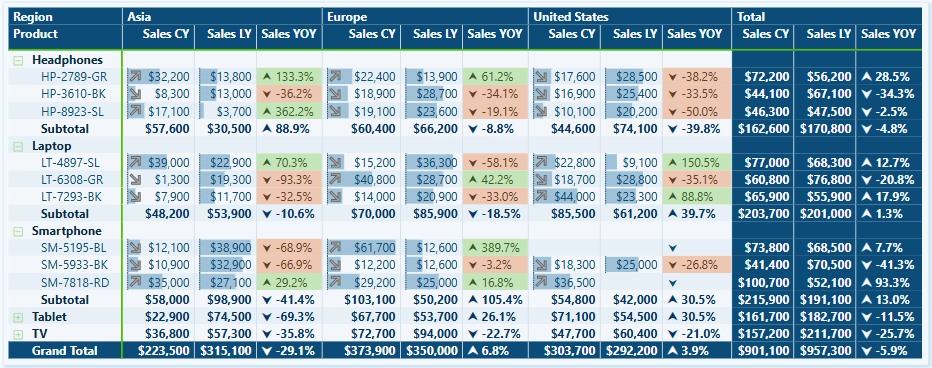
Example #1: % of Total (Within Selection vs Overall)

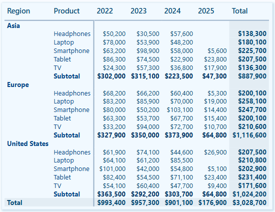
Our report presents the user with the total sales amounts for each region and product. But totals don’t always tell the story. Showing percentages helps answer two key questions quickly: How big is this option compared to the other? and How much does it contribute overall?

We can provide better insights at a glance by presenting a % of Total measure for each slicer option.

SVG Slicer % of Total = 
--% of Total (Within Selection vs Overall)

-- Base value calculated total sales for each value
VAR _contextTotal = [Sales Metric (CY)]
-- Total sales of the dimension within scope
VAR _selectedTotal = 
    SWITCH(
        TRUE(),
        ISINSCOPE(Regions[Region]),CALCULATE([Sales Metric (CY)], REMOVEFILTERS(Regions[Region])),
        ISINSCOPE(Products[Product]),CALCULATE([Sales Metric (CY)], REMOVEFILTERS(Products[Product]))
    )
-- Annual overall total sales
VAR _overallTotal = CALCULATE([Sales Metric (CY)], REMOVEFILTERS(Products[Product]), REMOVEFILTERS(Regions[Region]))
-- The two percentage calculations to show
VAR __percentageWithinSelection = DIVIDE(_contextTotal, _selectedTotal)
VAR _percentageOverall = DIVIDE(_contextTotal, _overallTotal)
-- Logic determining which calculation to show
---- Region Slicer and Products are filtered -> show within selection
---- Product Slicer and Regions are filtered -> show within selection
---- Otherwise -> show overall
VAR _percentageDisplay = 
    SWITCH(
        TRUE(), 
        //Regional Slicer Conditions
        ISINSCOPE(Regions[Region]) && ISFILTERED(Products), __percentageWithinSelection,
        //Products Slicer Conditions
        ISINSCOPE(Products[Product]) && ISFILTERED(Regions), __percentageWithinSelection,
        //Default
        _percentageOverall
    )
RETURN
    IF( 
        NOT ISBLANK(_percentageDisplay) && _percentageDisplay <> 0, 
        FORMAT(_percentageDisplay, "0.0%"), 
        "-–"
    )

To avoid confusion and clarify the meaning of each percentage within its current context, we also add the following measures to the subtitle property of our slicers.

SVG Slicer Region SubTitle = IF(ISFILTERED(Products), "% w/in Product Selection", "% Overall")

SVG Slicer Product SubTitle = IF(ISFILTERED(Regions), " % w/in Regional Selection", "% Overall")

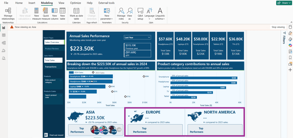
BONUS!: Curious about the Top Performers on the Regional data cards? Check out My Best Power BI KPI Card (So Far 😅) by Isabelle Bittar for the details!

Why show both “overall” and “within selection”?

• Overall answers: “How important or significant is this choice globally?” Helpful in spotting major contributors or outliers without any filtering required.
• Within selection answers: “Inside my current regional selection, how much does this item contribute or matter?” Perfect when users have already narrowed the context (e.g. filtered to a specific region and are now choosing products within it).

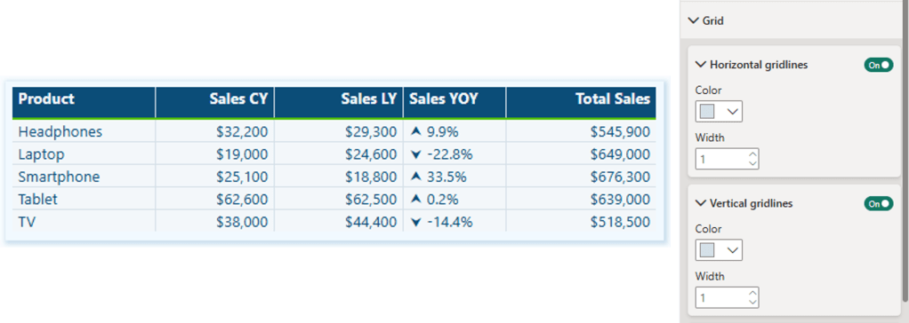
Example #2: Tracking Sales Trends

Totals and percentages show size and share, but they don’t show direction. By adding arrows and percent change to slicer items, users see momentum at a glance. What’s rising, what’s falling, and what’s holding steady.

Step #1: Calculating the 6-Month Trend

This measure compares sales from the past six months to those from the previous six months. The outcome is a percent change that serves as the basis for our trend indicator.

Sales Trend % (6M vs Prev 6M) = 
-- Trend preview (6M vs prior 6M)

-- Anchor date for the window (respects current filter context; falls back to max Sales date)
VAR _anchor = MAX(Sales[SalesDate])
-- Total sales for the last 6 months ending at the anchor date
VAR _last6m =
    CALCULATE ([Total Sales], DATESINPERIOD (DateTable[Date], _anchor, -6, MONTH))
-- Total sales for the prior 6 months (months -12 to -6 from the anchor)
VAR _prev6m =
    CALCULATE (
        [Total Sales],
        DATESBETWEEN (DateTable[Date], EDATE (_anchor, -12), EDATE (_anchor, -6))
    ) 

RETURN 
DIVIDE ( _last6m - _prev6m, _prev6m )

Step #2: Enhancing Percent Change With A Visual Indicator

Once we have identified the trend, the next step is to add a visual indicator to quickly determine whether the trend is moving up or down. A positive change is represented by an upward arrow, a negative change by a downward arrow, and any changes that fall within our defined noise band are indicated with a flat arrow.

SVG Slicer Trend Indicator = 
-- Render trend as arrow + % change label

-- Sales trend % from the prior measure
VAR _pct   = [Sales Trend % (6M vs Prev 6M)]
-- Noise band threshold (avoid flipping arrows on tiny changes)
VAR _band  = 0.02
-- Select arrow symbol based on trend direction
VAR _arrow =
    SWITCH ( TRUE(),
        ISBLANK ( _pct ),  "",
        _pct >  _band,     UNICHAR(11165),
        _pct < -_band,     UNICHAR(11167),
                           UNICHAR(11166)
    )
-- Format percentage text, fallback to “--” if blank
VAR pctTxt =
    IF (ISBLANK(_pct), "--", FORMAT(_pct, "0.0%"))
RETURN 
_arrow & " " & pctTxt

Step #3: Assigning Classes for Styling

To ensure our indicator remains readable across various slicer states (e.g. default, hover, pressed, selected), each state is assigned a simple class key: up, down, or flat. These keys correspond to different color rules in our SVG Slicer Styling measure.

SVG Trend Class Key = 
-- Assign trend class (up, down, flat) for slicer styling

-- Sales trend %
VAR pct  = [Sales Trend % (6M vs Prev 6M)]
-- Noise band threshold (avoid class flips on tiny changes)
VAR band = 0.02
-- Return class string for styling: up / down / flat
RETURN
    SWITCH ( TRUE(),
        ISBLANK ( pct ), "flat",
        pct >  band,     "up",
        pct < -band,     "down",
                         "flat"
    )

Step #4: Add Styling for State and Trend

Enhance the styling of our slicers by adding classes for trend and selection states. Defining these colors will ensure readability on both dark and light slicer backgrounds.

SVG Slicer Styling = 
"
<style>
.slicerTextDefault {
    font:9pt Segoe UI Regular; 
    fill:#9FC2D9;
    text-anchor:end; 
    alignment-baseline:middle
    }
.slicerTextHover {
    font:9pt Segoe UI Regular; 
    fill:#FFFFFF;
    text-anchor:end; 
    alignment-baseline:middle
    }
.slicerTextPressed {
    font:9pt Segoe UI Regular; 
    fill:#FFFFFF;
    text-anchor:end; 
    alignment-baseline:middle
    }
.slicerTextSelected {
    font:9pt Segoe UI Regular; 
    fill:#073450;
    text-anchor:end; 
    alignment-baseline:middle
    }

.up-default   { fill:#79D3B5; }  
.down-default { fill:#FFA19A; }  
.flat-default { fill:#BFD4E2; }

.up-hover     { fill:#79D3B5; }  
.down-hover   { fill:#FFA19A; }  
.flat-hover   { fill:#BFD4E2; }

.up-pressed   { fill:#79D3B5; }  
.down-pressed { fill:#FFA19A; }  
.flat-pressed { fill:#BFD4E2; }

.up-selected   { fill:#0F7B5F; }  
.down-selected { fill:#B23D33; } 
.flat-selected { fill:#4A6373; }
</style>
"

Step #4: Wrap Our Trend Indicator in our SVG Slicer Measures

Finally, we update our display measure, which determines what appears in our slicer. This wrapper combines the class key with the slicer’s state.

SVG Slicer Display = 
-- Display sales trend comparing the last 6M to the 6M prior 
    [SVG Slicer Trend Indicator] 

SVG Slicer Default = 
VAR _state = "default"
VAR _cls = [SVG Trend Class Key] & "-" & _state        
RETURN
"data:image/svg+xml;utf8,
<svg xmlns='http://www.w3.org/2000/svg'  viewBox='0 0 100% 100%'  >" & [SVG Slicer Styling] &"
<rect x='0' y='0' width='100%' height='100%' fill='transparent'> </rect>
<text x='100%' y='55%' class='slicerTextDefault " & _cls & "'>" &  [SVG Slicer Display] & "</text>
</svg>"

SVG Slicer Hover = 
VAR _state = "hover"
VAR _cls = [SVG Trend Class Key] & "-" & _state   
RETURN
"data:image/svg+xml;utf8,
<svg xmlns='http://www.w3.org/2000/svg'  viewBox='0 0 100% 100%'  >" & [SVG Slicer Styling] &"
<rect x='0' y='0' width='100%' height='100%' fill='transparent'> </rect>
<text x='100%' y='55%' class='slicerTextHover " & _cls & "'>" & [SVG Slicer Display] & "</text>
</svg>"

SVG Slicer Pressed = 
VAR _state = "pressed"
VAR _cls = [SVG Trend Class Key] & "-" & _state   
RETURN
"data:image/svg+xml;utf8,
<svg xmlns='http://www.w3.org/2000/svg'  viewBox='0 0 100% 100%'  >" & [SVG Slicer Styling] &"
<rect x='0' y='0' width='100%' height='100%' fill='transparent'> </rect>
<text x='100%' y='55%' class='slicerTextPressed " & _cls & "'>" &  [SVG Slicer Display] & "</text>
</svg>"

SVG Slicer Selected = 
VAR _state = "selected"
VAR _cls = [SVG Trend Class Key] & "-" & _state   
RETURN
"data:image/svg+xml;utf8,
<svg xmlns='http://www.w3.org/2000/svg'  viewBox='0 0 100% 100%'  >" & [SVG Slicer Styling] &"
<rect x='0' y='0' width='100%' height='100%' fill='transparent'> </rect>
<text x='100%' y='55%' class='slicerTextSelected " & _cls & "'>" &  [SVG Slicer Display] & "</text>
</svg>"

Why This Matters

By incorporating trend indicators directly into the slicer, users can see not only the magnitude of sales but also the momentum behind them. A mid-level product that is experiencing rising sales can stand out just as much as a top seller in decline. This additional context helps focus attention on what is changing, rather than just what is popular.

Slicers can be more than just passive filters in our reports. By incorporating a few DAX measures and some simple SVG styling, we can transform them into interactive visuals that provide insights and help users better understand their selections. Since our reports have limited canvas space, enhancing our slicers with these features enables us to utilize the entire canvas area effectively.

The next time you add a slicer, consider going beyond a simple list. Consider how the slicer can facilitate a dynamic interaction with the data, helping to inform decisions and answer key questions before users take action. This subtle design shift can significantly enhance users’ ability to explore our reports.

The example report can be found at the link below!

GitHub – Design Meets Data

A practical series on blending UX and analytics in Power BI. Each entry includes a working PBIX and sample data so you can explore design patterns directly in your own environment.

Thank you for reading! Stay curious, and until next time, happy learning.

And, remember, as Albert Einstein once said, “Anyone who has never made a mistake has never tried anything new.” So, don’t be afraid of making mistakes, practice makes perfect. Continuously experiment, explore, and challenge yourself with real-world scenarios.

If this sparked your curiosity, keep that spark alive and check back frequently. Better yet, be sure not to miss a post by subscribing! With each new post comes an opportunity to learn something new.

Type your email…

Subscribe