Elevate Your Power BI Reports with Context-Aware Insights
Welcome, to another journey through the world of DAX, in this post we will be shining the spotlight on the ISINSCOPE function. If you have been exploring DAX and Power BI you may have encountered this function and wondered its purpose. Well, wonder no more! We are here to unravel the mysteries and dive into some practical example showing just how invaluable this function can be in our data analysis endeavors.
If you are unfamiliar DAX is the key that helps us unlock meaningful insights. It is the tool that lets us create custom calculations and serve up exactly what we need. Now, lets focus on ISINSCOPE, it is a function that might not always steal the show but plays a pivotal role, particularly when we are dealing with hierarchies and intricate drilldowns in our reports. It provides us the access to understand at which level of hierarchy our data is hanging out, ensuring our calculations are always in tune with the context.
For those of you eager to start experimenting there is a Power BI report pre-loaded with the sample data used in this post ready for you. So don’t just read, follow along and get hands-on with DAX in Power BI. Get a copy of the sample data file (power-bi-sample-data.pbix) here:
This dynamic repository is the perfect place to enhance your learning journey.
Exploring the ISINSCOPE Function
Let’s dive in and get hand on with the ISINSCOPE function. Think of this function as our data GPS, it helps us figure out where we are in the grand scheme of our data hierarchies.
So, what exactly is ISINSCOPE? In plain terms, it is a DAX function used to determine if a column is currently being used in a specific level of a hierarchy or, put another way, if we are grouping by the column we specify. The function returns true when the specified column is the level being used in a hierarchy of levels. The syntax is straightforward:
ISINSCOPE(column_name)
The column_name argument is the name of an existing column. Just add a column that we are curious about, and ISINSCOPE will return true or false depending on whether that column is in the current scope.
Let’s use a simple matrix containing our Region, Product Category, and Product Code to set up a hierarchy and see ISINSCOPE in action with the following formula.
This formula uses ISINSCOPE in combination with SWITCH to determine the current context, and if true returns a text label indicating what level is in context.
But why is this important? Well, when we are dealing with data, especially in a report or a dashboard, we want our calculations to be context-aware. We want them to adapt based on the level of data we are looking at. ISINSCOPE allows us to create measures and calculated columns that behave differently at different levels of granularity. This helps provide accurate and meaningful insights.
Diving Deeper: How ISINSCOPE Works
Now that we have got a handle on what ISINSCOPE is, let’s dive a bit deeper and see how it works. At the heart of it ISINSCOPE is all about context, specifically, row context and filter context.
For an in depth look into Row Context and Filter Context check out the posts below that provide all the details.
Filter Context – How to create it and its impact on measures
For our report we are interested in analyzing the last sales date of our products, and want this information in a matrix similar to the example above. We can easily create a Last Sales Date measure using the following formula and add it to our matrix visual.
Last Sales Date = MAX(Sales[SalesDate])
This provides a good start, but not quite what we are looking for. For our analysis the last sales date at the Region level is too broad and not of interest, while the sales date of Product Code is too granular and clutters the visual. So, how do we display the last sales date just at the Product Category (e.g. Laptop) level? Enter ISINSCOPE.
Let’s update our Last Sales Date measure so that it will only display the date on the product category level. Here is the formula.
Product Last Sales Date =
SWITCH(
    TRUE(),
    ISINSCOPE(Products[Product Code]), BLANK(),
    ISINSCOPE(Products[Product]), FORMAT(MAX(Sales[SalesDate]),"MM/dd/yyyy"),
    ISINSCOPE(Regions[Region]), BLANK()
)
We use SWITCH in tandem with ISINSCOPE to determine the context, and if Product is in context the measure returns the last sales date for that product category. However, at the Region and Product Code levels the measure will return a blank value.
The use of ISINSCOPE helps enhance the matrix visual preventing it from getting over crowded with information and ensuring that the information displayed is relevant. It acts as a smart filter, showing or hiding data based on where we are in a hierarchy, making our reports more intuitive and user-friendly.
ISINSCOPE’s Role in Hierarchies and Drilldowns
When we are working with data, understanding the relationship between parts and the whole is crucial. This is where hierarchies and drilldowns come into play, and ISINSCOPE is the function that helps us make sense of it all.
Hierarchies allow us to organize our data in a way that reflects real-world relationships, like breaking down sales by region, then product category, then specific products. Drilldowns let us start with a broad view and then zoom in on the details. But how do we keep our calculations accurate at each level? You guessed it, ISINSCOPE.
Let’s look at a DAX measure that leverages ISINSCOPE to calculate the percentage of sales each child represents of the parent in our hierarchy.
Percentage of Parent =
    VAR AllSales =
        CALCULATE(Sales[Total Sales], ALLSELECTED())
    VAR RegionSales =
        CALCULATE([Total Sales], ALLSELECTED(), VALUES(Regions[Region]))
    VAR RegionCategorySales =
        CALCULATE([Total Sales], ALLSELECTED(), VALUES(Regions[Region]), VALUES(Products[Product]))
    VAR CurrentSales = [Total Sales]

RETURN
SWITCH(TRUE(),
    ISINSCOPE(Products[Product Code]), DIVIDE(CurrentSales, RegionCategorySales),
    ISINSCOPE(Products[Product]), DIVIDE(CurrentSales, RegionSales),
    ISINSCOPE(Regions[Region]), DIVIDE(CurrentSales, AllSales)
)
The Percentage of Parent measure uses ISINSCOPE to determine the current level of detail we are working with. If we are viewing our sales by region the measure calculates the sales for the region as a percentage of all sales.
But the true power of ISINSCOPE begins to reveal itself as we drilldown into our sales data. If we drilldown into each region to show the product categories we see that the measure will calculate the sales for each product category as a percentage of sales for that region.
And then again, if we drilldown into each product category we can see the measure will calculate the the sales of each product code as a percentage of sales for that product category within the region.
By incorporating this measure into our report, we help ensure that as we drilldown into our data the percentages are always calculated relative to the appropriate parent in our hierarchy. This allows us to provide accurate measures that provide the appropriate context, making our reports more intuitive and insightful.
ISINSCOPE is the key element to maintaining the integrity of our hierarchical calculations. It ensures that as we navigate through different levels of our data our calculations remain relevant and precise, providing a clear understanding of how each part contributes to the whole.
Best Practices for Leveraging ISINSCOPE
When it comes to DAX and ISINSCOPE a few best practices can ensure that our reports are accurate, performant, and user-friendly. Here are just a few things that can help us make the most out of ISINSCOPE:
Understand Context: Before using ISINSCOPE, make sure to have a solid understanding of row and filter context. Knowing which context we are working with will help us use ISINSCOPE effectively.
Keep it Simple: Start with simple measures to understand how ISINSCOPE behaves with our data. Complex measures can be built up gradually as we become more comfortable with the function.
Use Variables: Variables can make our DAX formulas easier to read and debug. They also help with performance because they store a result of a calculation for reuse.
Test at Every Level: When creating measures with ISINSCOPE, test them at every level, this helps ensure that our measures work correctly no matter how the users interact with the report.
Combine with Other Functions:ISINSCOPE is often used in combination with other DAX functions. Learning how it interacts with functions like SWITCH, CALCULATE, FILTER, and ALLSELECTED will provide us more control over our data.
Wrapping up
Throughout our exploration of the ISINSCOPE function we have uncovered its pivotal role in managing data hierarchies and drilldowns providing for accurate and context-sensitive reporting. Its ability to discern the level of detail we are working with allows for dynamic measures and visuals that adapt to user interactions, making our reports not just informative but interactive and intuitive.
With practice, ISINSCOPE will become a natural part of your DAX toolkit, enabling you to create sophisticated reports that meet the complex needs of any data analysis challenge you might face.
For those looking to continue their journey into DAX and its capabilities there is a wealth of resources available, and a good place to start is the DAX Reference documentation.
Learn more about: Power Automate Excel Online (Business) Actions
I have also written about other DAX functions including Date and Time Functions, Text Functions, an entire post focused on the CALCULATE function and an ultimate guide providing a overview of all the DAX function groups.
Unlock the Full Potential of Your Data with DAX: From Basic Aggregations to Advanced Time Intelligence
Thank you for reading! Stay curious, and until next time, happy learning.
And, remember, as Albert Einstein once said, “Anyone who has never made a mistake has never tried anything new.” So, don’t be afraid of making mistakes, practice makes perfect. Continuously experiment and explore new DAX functions, and challenge yourself with real-world data scenarios.
If this sparked your curiosity, keep that spark alive and check back frequently. Better yet, be sure not to miss a post by subscribing! With each new post comes an opportunity to learn something new.
Explore the ebb and flow of the temporal dimension of your data with DAX’s suite of Date and Time Functions.
In data analysis, understanding the nuances of time can be the difference between a good analysis and a great one. Time-based data, with its intricate patterns and sequences offers a unique perspective into trends, behaviors, and potential future outcomes. DAX provides specialized date and time functions helping guide us through the complexities of temporal data with ease.
Curious what this post will cover? Here is the break down, read top to bottom or jump right to the part you are most interested in.
For those of you eager to start experimenting there is a Power BI report pre-loaded with the sample data used in this post ready for you. So don’t just read, following along and get hands-on with DAX in Power BI. Get a copy of sample data file (power-bi-sample-data.pbix) here:
This dynamic repository is the perfect place to enhance your learning journey and serves as an interactive compliment to the blog posts on EthanGuyant.com.
The Power of Date and Time in Data Analysis
Consider the role of a sales manager for a electronic store. Knowing 1,000 smartphones were sold last month provides a good snapshot. But, understanding the distribution of these sales-like the surge during weekends or the lull on weekdays-offers greater insights. This level of detail is made possible by time-based data and allows for more informed decisions and strategies.
DAX and Excel: Spotting the Differences
For many, the journey into DAX begins with a foundation in Excel and the formulas it provides. While DAX and Excel share a common lineage, they two have distinct personalities and strengths. Throughout this post if you are familiar with Excel you may recognize some functions but it is important to note that Excel and DAX work with dates differently.
Both DAX and Excel boast a rich array of functions, many of which sound and look familiar. For instance the TODAY() function exists in both. In Excel, TODAY() simply returns the current date. In DAX, while TODAY() also returns the current date it does so within the context of the underlying data model, allowing for more complex interactions and relationships with other data in Power BI.
Excel sees dates and times as serial numbers, a legacy of its spreadsheet origins. DAX, on the other hand, elevates them with a datetime data type. This distinction means that in DAX, dates and times are not just values, they are entities with relationships, hierarchies, and attributes. This depth allows for a range of calculations in DAX that would require workarounds in Excel. And with DAX’s expansive library of date time functions, the possibilities are vast.
For more details on DAX date and time functions keep reading and don’t forget to also checkout the Microsoft documentation.
Diving into DAX can fell like like stepping into the ocean. But fear not! Let’s wade into the shallows first by getting familiar with some basic functions. These foundational functions will set the stage for more advanced explorations later on.
DATE: Crafting Dates in Datetime Formats
The DATE function in DAX is a tool for manually creating dates. It syntax is:
DATE(year, month, day)
As you might expect, year is a number representing the year. What may not be as clear is the year argument can include one to four digits. Although years can be specified with two digits it best practice to use four digits whenever possible to avoid unintended results. For example:
Use Four Digit Years = DATE(23, 1, 1)
Will return January 1st, 1923, not January 1st, 2023 as may have been intended.
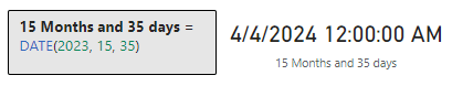
The month argument is a number representing the month, if the value is a number from 1 to 12 then it represents the month of the year (1-January, …, 12-December). However, if the value is greater than 12 a calculation occurs. The date is calculated by adding the value of month to January of the specified year. For example, using DATE if we specify the year as 2023 and the month as 15, we will get a results for March 2024.
15 Months = DATE(2023, 15, 1)
Similarly the argument day is a number representing the day of the month or a calculation. The day argument results in a calculation if the value is greater than the last day of the given month, otherwise it simply represents the day of the month. The calculation is similar to how the month argument works, if day is greater than the last day of the month the value is added to month. If we take the example above and change day to be 35, we can see it returns a date of April 4th, 2024.
DAY, MONTH, YEAR: Extracting Date Components
Sometimes, we just need a piece of the date. Whether it is the day, month, or year, DAX has a function for that. All of these functions have similar syntax and have a singular date argument which can be a date in datetime format or text format (e.g. “2023-01-01”).
DAY(date)
MONTH(date)
YEAR(date)
Note: At the time of writing today is 10/20/2023. The TODAY() function is used through out this post.
These functions are pivotal when segmenting data, creating custom date hierarchies, or performing year-over-year and month-over-month analyses.
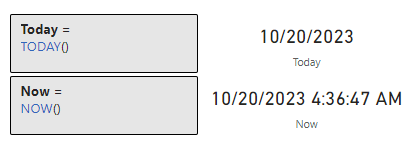
TODAY and NOW: Capturing the Present Moment
In the dynamic realm of data, real-time insights are invaluable. The TODAY function in DAX delivers the current date without time details. It is perfect for age calculations or determining days since a particular event. Conversely, NOW provides a detailed timestamp, including the current time. This granularity is essential for monitoring live data, event logging, or tracking activities.
The examples above provide examples of using TODAY, the below example highlights the differences between TODAY and NOW.
With these foundational date functions in our tool box we are equipped to continue deeper into DAX’s date and time capabilities. These might seem basic, but their adaptability and functionality are the bedrock for more complex and advanced operations and analyses.
Diving Deeping: Advanced Date Manipulations
As we become more comfortable with DAX’s basic date functions you may begin to wonder what more can DAX’s Date and Time functions do. Diving deeper into DAX’s date functions we will discover more advanced tools specific to addressing date-related challenges. Whether it is shifting dates, pinpointing specific moments, or calculating intervals, DAX’s date and time functions are here to elevate our data analysis and conquer these challenges.
EDATE: Shifting Dates by Month
A common challenge we may encounter is the need to project a date a few months into the future or trace back to a few months prior. EDATE is the function for the job, EDATE allows us to shift a date by a specified number of months. The syntax is:
EDATE(start_date, months)
The start_date is a date in datetime or text format and is the date that we want to shift by the value of months. The months argument is an integer representing the number of months before or after the start_date. One thing to note is that if the start_date is provided in text format the function will interpret this based on the locale and date time settings of the client computer. For example if start_date is 10/1/2023 and the date time settings represent a date as Month/Day/Year this will be interpreted as October 1st, 2023, however if the date time settings represent a date as Day/Month/Year it will be interpreted as January 10th, 2023.
For example, say we follow up on a sale or have a business process that kicks off 3 months following a sale. We can use EDATE to project the SalesDate and identify when this process should occur. We can use:
3 Months after Sale = EDATE(MAX(Sales[SalesDate]), 3)
EOMONTH: Pinpointing the Month’s End
End-of-month dates are crucial for a variety of purposes. With EOMONTH we can easily determine the last date of a month. The syntax is the same as EMONTH:
EOMONTH(start_date, months)
We can use this function to identify the end of the month for each of our sales.
Sales End of Month = EOMONTH(MAX(Sales[SalesDate]), 0)
In the example above we use 0 to indicate we want the end of the month in which the sale occurred. If we needed to project the date to the end of the following month we would update the months argument from 0 to 1.
DATEDIFF & DATEADD: Date Interval Calculations
The temporal aspects of our data can be so much more than static points on a timeline. They can represent intervals, durations, and sequences. By understanding the span between dates or manipulating these intervals we can provide additional insights required by our analysis.
DATEDIFF is the function to use when measuring the span between two dates. With this function we can calculate the age of an item, or the duration of a project. DATEDIFF calculates the difference between the dates base on days, months, or years. Its syntax is:
DATEDIFF(date_1, date_2, interval)
The date_1 and date_2 arguments are the two dates that we want to calculated the difference between. The result will be a positive value if date_2 is larger than date_1, otherwise it will return a negative result. The interval argument is the interval to use when comparing the two dates and can be SECOND, MINUTE, HOUR, DAY, WEEK, MONTH, QUARTER, or YEAR.
We can use DATEDIFF and the following formula to calculate how many days it has been since our last sale, or the difference between our last Sales date and Today.
Days Between Last Sale and Today =
DATEDIFF(MAX(Sales[SalesDate]), TODAY(), DAY)
The above example shows as of 10/20/2023 it has been 64 days since our last sale.
In the DATE: Crafting Dates in Datetime Format section we saw that providing DATE a month value greater than 12 or a day value greater than the last day of the month will add values to the year or month. However, if the goal is to adjust our dates by an specific interval the DATEADD function can be much more useful. Although in the DAX Reference documentation DATEADD is categorized under Time Intelligence functions it is still helpful to mention here. The syntax for DATEADD is:
DATEADD(dates, number_of_intervals, interval)
The dates argument is a column that contains dates. The number_of_intervals is an integer that specifies the number of intervals to add or subtract. If number_of_intervals is positive the calculation will add the intervals to dates and if negative it will subtract the intervals from dates. Lastly, interval is the interval to adjust the dates by and can be day, month, quarter, or year. For more details and examples on DATEADD checkout my previous post Time Travel in Power BI: Mastering Time Intelligence Functions.
Journey through the Past, Present, and Future of Your Data with Time Intelligence Functions.
Advanced date manipulations in DAX open up a world of possibilities. From forecasting and backtracking to pinpointing specific intervals. These functions empower us to navigate the intricacies of our data providing clarity and depth to our analysis.
Times Ticking: Harnessing DAX Time Functions
In data analysis, time is so much more than just ticking seconds on a clock. Time provides an element of our data to help understand its patterns looking back, or predicting trends looking forward. DAX provides us a suite of time functions that allow us to dissect, analyze, and manipulate time data.
HOUR, MINUTE, and SECOND: Breaking Down Time Details
Time is a composite of hours, minute, and seconds. DAX provides individual functions that extract each of these components.
As you might have expected these functions are appropriately named HOUR, MINUTE, and SECOND. They also all follow the same general syntax.
HOUR(datetime)
MINUTE(datetime)
SECOND(datetime)
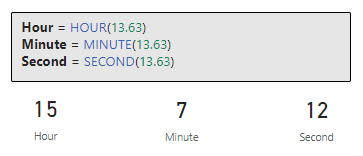
Each function then returns its respective time component, HOUR will return a value from 0 (12:00AM) to 23 (11:00PM), MINUTE returns a value from 0 to 59, and SECOND returns a value also from 0 to 59.
All of these functions take the datetime that contains the component we want to extract as the singular argument. The time can be supplied using datetime format, another expression that returns a datetime (e.g. NOW()), or text in an accepted time format. When the datetime is provided as text the function uses the locale and datetime setting of the client computer to interpret the text value. Most locales use a colon : as the time separator and any text input using colons will parse correctly.
It is also important to be mindful when these functions are provided a numeric value to avoid unintended results. The serial number will first be represented as a datetime data type before the time component is extracted. To more easily understand the results of our calculations its best to first represent these values as datetime data types before passing them to the functions. For example, passing a value of 13.63 to the HOUR function will return a value of 15. This is because 13.63 is first represented as a datetime 1/13/1900 15:07:12 and then the time components are extracted.
TIMEVALUE: Converting Text to Time
In our datasets time values might sometimes be stored as text. The TIMEVALUE function is the go to tool for handling these text values. This function will convert a text representation of time (e.g. "18:15") into a time value. Applying TIMEVALUE converts the text to a time value making it usable for time-based calculations.
Text to Time = TIMEVALUE("18:15")
DAX’s time functions allow us to zero in on the details of our datetime data. When we need to segment data by hours, set benchmarks, or convert time formats, these functions ensure we always have the tools ready to address these challenges.
Special DAX Functions for Date and Time
Dates and times a crucial parts of many analytical tasks. DAX offers a wide array of specialized functions that cater to unique date and time requirements helping us ensure we have the proper tools needed for every analytical challenge we face.
CALENDAR and CALENDARAUTO: Generating a Date Table
When developing our data model having a continuous date table can be an invaluable asset. DAX provides two functions that can help us generate date table within our data model.
CALENDAR will create a table with a single “Date” column containing a contiguous set of dates starting from a specified start date and ending at a specified end date. The syntax is:
CALENDAR(start_date, end_date)
The range of dates is specified by the two arguments and is inclusive of these two dates. CALENDAR will result in an error if start_date is greater than end_date.
CALENDARAUTO takes CALENDAR one step further by adding some automation. This function will generate a date table based on the data already in our data model. It identifies the earliest and latest dates and creates a continuous date table accordingly. When using CALENDARAUTO we do not have to manually specify the start and end date, here is the functions syntax:
CALENDARAUTO([fiscal_year_end_month])
The CALENDARAUTO function has a single optional argument fiscal_year_end_month. This argument can be used to specify the month the year ends and can be a value from 1 to 12. If omitted the default value will be 12.
A few things to note about the automated calculation. The start and end dates are determined by dates in the data model that are not in a calculated column or a calculated table and the function will generate an error if no datetime values are identified in the data model.
NETWORKDAYS: Calculating Workdays Between Two Dates
In business scenarios, understanding workdays is crucial for tasks like planning or financial forecasting. The NETWORKDAYS functions calculates the number of whole workdays between two dates, excluding weekends and providing the options to exclude holidays. The syntax is:
The start_date and end_date are the dates we want to know how many workdays are between. Within the NETWORKDAYS the start_date can be earlier than, the same as, or later than the end_date. If start_date is greater than end_date the function will return a negative value. The weekend argument is optional and is a weekend number which specifies when the weekends occur, for example a value of 1 (or if omitted) indicates the weekend days are Saturday and Sunday. Check out the parameter details for a list of all the options.
Lastly, holidays is a column table of one or more dates that are to be excluded from the working day calendar.
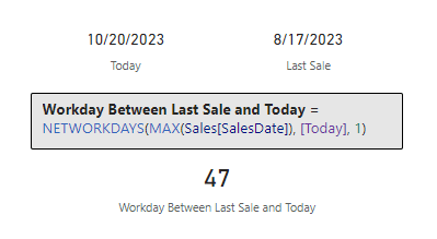
Let’s take a look at an example, from our previous Days Between Last Sale and Today example we know there at 64 days since our last sale. Let’s use the following formula to identify how many of those are workdays.
Workday Between Last Sale and Today =
NETWORKDAYS(MAX(Sales[SalesDate]), [Today], 1)
Note: At the time of writing the last sales date is 8/17/2023 and today is 10/20/2023
Taking into account the date range noted above, we can update the Workday Between Last Sale and Today to exclude Labor Day (9/4/2023) using this updated formula.
Workday Between Last Sale and Today (No Holidays) =
NETWORKDAYS(
    MAX(Sales[SalesDate]),
    [Today],
    1,
    {DATE (2023, 9, 4)}
)
QUARTER and WEEKDAY: Understanding Date Hierarchies
When we need to categorized our dates into broader hierarchies functions like QUARTER and WEEKDAY can help with this task. QUARTER returns the quarter of the specified date and returns a number from 1 to 4.
QUARTER(date)
WEEKDAY provides the day number of the week ranging from 1(Sunday) to 7 (Saturday) by default.
WEEKDAY(date, return_type)
The date argument should be in datetime format and entered by using the DATE function or by another expression which returns a date. The return_type determines what value is returned, a value of 1 (or omitted) indicates the week begins on Sunday (1) and ends Saturday (7), 2 indicates the week begins Monday (1) and ends Sunday (7), and 3 the week begins Monday (0) and ends Sunday (6).
Let’s take a look at the WEEKDAY function and return_type by using the following formulas to evaluate Monday, 10/16/2023.
DAX’s specialized date and time functions are helpful tools designed just for us. They cater to the unique requirements of working with date and times, ensuring that we are set to tackle any analytical challenge we may face with precision and efficiency.
Yearly Insights with DAX
The annual cycle holds significance in numerous domains, from finance to academia. Yearly reviews, forecasts, and analyses form the cornerstone of many decision-making processes. DAX offers a set of functions to extract and manipulate year-related data, ensuring you have a comprehensive view of annual trends and patterns.
We have already explored the first function that provides yearly insights, YEAR. This straightforward yet powerful function extracts the year from a given date and allows us to categorize or filter data based on the year. Let’s explore some other DAX functions that help provide us yearly insights into our data.
YEARFRAC: Computing the Year Fraction Between Dates
Sometimes, understanding the fraction of a year between two dates can be beneficial. The YEARFRAC function calculates the fraction of a year between two dates. The syntax is:
YEARFRAC(start_date, end_date[, basis])
Same as other date functions start_date and end_date are the dates we are interested in knowing the fraction of a year between and they are passed to YEARFRAC in datetime format. The basis argument is optional and is the type of day count basis to be used for the calculation. The default value is 0 and indicates the use of US (NASD) 30/360. Other options include 1-actual/actual, 2-actual/360, 3-actual/365, and 4-European 30/360.
Let’s examine the difference between our last sale and today again. From our previous calculation we know there is 64 days between our last sale and today (10/23/2023), we can use YEARFRAC to represent this difference as a fraction of a year.
Fraction of Year Between Last Sale and Today =
YEARFRAC(MAX(Sales[SalesDate]), TODAY(), 0)
WEEKNUM: Determining the Week Number of a Date
Our analysis in many scenarios may require or benefit from understanding weekly cycles. The WEEKNUM function gives us the week number of the specified date, helping us analyze data on a weekly basis. The syntax for WEEKNUM is
WEEKNUM(date[, return_type])
The return_type argument is optional and represents which day the week begins. The default value is 1 indicating the week begins on Sunday.
An important note about WEEKNUM is that the function uses a calendar convention in which the week that contains January 1st is considered to be the first week of the year. However, the ISO 8601 calendar standard defines the first week as the one that has four or more days (contains the first Thursday) in the new year, if this standard should be used the return_type should be set to 21. Check out the Remarks section of the DAX Reference for details on available options.
Let’s explore the differences between using the default return_type where week one is the week which contains January 1st, and a return_type of 21 where week one is the first week that has four or more days in it (with the week starting on Monday). To do this we will fast forward to Wednesday January 6th, 2027.
In 2027 January 1st lands on a Friday, so using Monday as the start of the week results in 3 days in 2027 being in that week and the first week in 2027 with four or more days (or containing the first Thursday) begins Monday, January 4th.
Harnessing the power of these functions allows us to dive deep into annual trends, make better predictions, and craft strategies that resonate with the yearly ebb and flow of our data.
Wrapping Up Our DAX Temporal Toolkit Journey
Time is a foundational element in data analysis. From understanding past trends to predicting future outcomes, the way we interpret and manipulate time data can significantly influence our insights. DAX offers a robust suite of date and time functions, providing a comprehensive toolkit to navigate the temporal dimensions of our data.
As business continue to trend toward being more data-driven, the need for precise time-based calculations will continue to grow. Whether it is segmenting sales data by quarters, forecasting inventory based on past trends, or understanding productivity across different time zones, DAX provides us the tools to tackle these tasks.
For those looking to continue this journey into DAX and its capabilities there is a wealth of resources available, and a good place to start is the DAX Reference documentation.
Learn more about: Power Automate Excel Online (Business) Actions
I have also written about other DAX function groups including Time Intelligence functions, Text Functions, an entire post focused on CALCULATE and an ultimate guide providing a overview of all the DAX function groups.
Unlock the Full Potential of Your Data with DAX: From Basic Aggregations to Advanced Time Intelligence
In the end, dates are more than just numbers on a calendar and time is more than just ticks on a clock. They are the keys to reveal the story of our data. With the power of DAX Date and Time Functions we will be able to tell this story with ease and in the most compelling way possible.
Thank you for reading! Stay curious, and until next time, happy learning.
And, remember, as Albert Einstein once said, “Anyone who has never made a mistake has never tried anything new.” So, don’t be afraid of making mistakes, practice makes perfect. Continuously experiment and explore new DAX functions, and challenge yourself with real-world data scenarios.
If this sparked your curiosity, keep that spark alive and check back frequently. Better yet, be sure not to miss a post by subscribing! With each new post comes an opportunity to learn something new.
Stringing Along with DAX: Dive Deep into Text Expressions
Ever felt like your data was whispering secrets just beyond your grasp? Dive into the world of DAX Text Functions and turn those whispers into powerful narratives. Unlock stories hidden within text strings, and let your data weave tales previously untold.
Introduction to DAX Text Functions
We live in a world that’s overflowing with data. But let’s remember: data can be so much more than just numbers on a spreadsheet. It can be the letters we string together, and the words we read. Get ready to explore the exciting world of DAX Text Functions!
If you have ever worked with Power BI, you are likely familiar with DAX or Data Analysis Expressions. If you are new to Power BI and DAX check out these blog posts to get started:
Are you ready to take your data analysis to the next level?
DAX is the backbone that brings structure and meaning to the data we work with in Power BI. Especially when we are dealing with textual data, DAX stands out with its comprehensive set of functions dedicated just for this purpose.
So whether you’re an experienced data analyst or a beginner just starting your journey, you have landed on the right page. Prepare to explore the depth and breadth of DAX Text Functions. This is going to be a deep dive covering various functions, their syntax, and plenty of of examples!
For those of you eager to start experimenting there is a Power BI report loaded with the sample data used in this post ready for you. So don’t just read, dive in and get hands-on with DAX Functions in Power BI. Check out it here:
This dynamic repository is the perfect place to enhance your learning journey.
LEFT, RIGHT, & MID — The Text Extractors
Starting with the basics, LEFT, RIGHT, and MID. Their primary role is to provide tools for selectively snipping portions of text, enabling focused data extraction. Let’s go a little deeper and explore their nuances.
LEFT Function: As the name subtly suggests, the LEFT function fetches a specific number of characters from the start, or leftmost part, of a given text string.
The syntax is as simple as:
LEFT(text, number_of_characters)
Here, text is the text string containing the characters you want to extract, and number_of_characters is an optional parameter that indicates the number of characters you want to extract. It defaults to a value of 1 if a value is not provided.
RIGHT Function: The RIGHT function, mirrors the functionality of LEFT and aims to extract the characters from the end of a string, or the rightmost part.
MID Function: Now we have the MID function. This is the bridge between LEFT and RIGHT that doesn’t restrict you to the start or end of the text string of interest. MID enables you to pinpoint a starting position and then extract a specific number of characters from there.
The syntax is as follows:
MID(text, start_number, number_of_characters)
Here, text is the text string containing the characters you want to extract, start_number is the position of the first character you want to extract (positions in the string start at 1), and number_of_characters is the number of characters you want to extract.
Practical Examples: Diving Deeper with the Text Extractors
Let’s dive deeper with some examples. Let’s say we have a Product Code column within our Product Table. The Product Code takes the form of product_abbreviation-product_num-color_code for example, SM-5933-BK.
We will first extract the first two characters using LEFT, these represent the product abbreviation. We can create a calculated column in the products table using the following expression:
Product Abbrev = LEFT(Products[Product Code], 2)
Next, let’s use RIGHT to extract the last two characters which represent the color code of the product. We will add another calculated column to the products table using the following:
Product Color = RIGHT(Products[Product Code], 2)
Lastly, to pinpoint the unique product number which is nestled in the middle we will use MID. We add another calculated column to the products table using this expression:
Product Number = MID(Products[Product Code], 4, 4)
Together, these three functions form the cornerstone of text extraction. However, they can sometimes stumble when there are unexpected text patterns. Take, for instance, the last row shown below for Product Code TBL-57148-BLK.
You might have noticed that the example expressions above may not always extract the intended values due to their reliance on hardcoded positions and number of characters. This highlights the importance of flexible and dynamic text extraction methods.
Enter FIND and SEARCH! As we venture further into this post, we will uncover how these functions can provide much-needed flexibility to our extractions, making them adaptable to varying text lengths and structures. So, while the trio of LEFT, RIGHT, and MID are foundational, there is a broader horizon of DAX Text Functions to explore.
So, don’t halt your DAX journey here; continue reading and discover the expanded universe of text manipulation tools. Dive in, and let’s continue to elevate your DAX skills.
FIND & SEARCH — Navigators of the Text Terrain
In the landscape of DAX Text Functions, FIND and SEARCH stand out as exceptional navigators, aiding you in locating a substring within another text string. Yet, despite their apparent similarities, they come with clear distinctions that could greatly impact your results.
FIND Function: the detail-oriented one of the two functions. It is precise, and is case-sensitive. So, when using FIND, ensure you embrace the details and match the exact case of the text string you are seeking.
Here, find_text is the text string you are seeking, you can use empty double quotes "" to match the first character of within_text. Speaking of, within_text is the text string containing the text you want to find.
The other parameters are optional, start_number is the position in within_text to start the seeking and defaults to 1 meaning the start of within_text. Lastly, NotFoundValue although optional is highly recommended and represents the value the function will use when find_text is not found in within_text, typical values include 0, -1.
Note: if NotFoundValue is not specified and is not found in the function will return and error.
SEARCH Function: SEARCH is the more laid-back of the two functions. It is adaptable and does not account for case, whether it’s upper case, lower case or a mix SEARCH will find the text you are looking for.
When combined with LEFT, RIGHT, or MID the potential of FIND and SEARCH multiplies, allowing for dynamic text extraction. Let’s consider the problematic Product Code TBL-57148-BLK again.
We started by extracting the product abbreviation with the following expression:
Product Abbrev = LEFT(Products[Product Code], 2)
This works well when all the product codes start with a two-letter abbreviation. But what if they don’t? The fixed number of characters to extract might yield undesirable results. Let’s use FIND to add some much-needed flexibility to this expression.
We know that the product abbreviation is all the characters before the first hyphen. To determine the position of the the first hyphen we can use:
First Hyphen = FIND("-", Products[Product Code])
For TBL-57148-BLK this will return a value of 4. We can then use this position to update our expression to dynamically extract the product abbreviation.
Next, let’s add some adaptability to our Product Color expression to handle when the color code may contain more than two characters. We started with the following expression:
Product Color = RIGHT(Products[Product Code], 2)
This expression assumes that all product color codes are consistently placed at the end and always two characters. However, if there are variations in the length (e.g. TBL-57148-BLK) this method might not be foolproof. To introduce some adaptability, let’s utilize SEARCH.
To determine the position of the last hyphen, since the color code will always be all the characters following this we can use:
Here, for the start_number we use the same FIND expression that we did to locate the first hyphen and then add 1 to the position to start the search for the second.
With this position, we can update our Product Color function to account for potential variations:
Product Color Dynamic =
VAR _firstHyphenPosition =
    FIND (
        "-",
        Products[Product Code]
    )
VAR _lastHyphenPosition =
    SEARCH (
        "-",
        Products[Product Code],
        _firstHyphenPosition + 1
    )
RETURN
    RIGHT (
        Products[Product Code],
        LEN ( Products[Product Code] ) - _lastHyphenPosition
    )
The updated calculated column finds the position of the first hyphen, and then uses this position to search for the position of the last hyphen. Once we know the position, we can use this position and the length of the string to determine the number of characters needed to extract the color code ( LEN(Products[Product Code]) - _lastHyphenPosition).
Through the use of FIND, SEARCH, and RIGHT, the DAX text extraction becomes more adaptable, and handles even unexpected product code formats with ease.
Similarly, we can update the the Product Number expression to:
Through these examples we have highlighted how to build upon the basics of LEFT, RIGHT, and MID by amplifying their flexibility through the use of FIND and SEARCH.
When it comes to locating specific strings within a text string, both FIND and SEARCH offer a helping hand. But, as is often the case with DAX, the devil is in the details. While they seem quite similar at a glance, a deeper exploration uncovers unique traits that set them apart. What’s main difference? Case sensitivity.
Let’s explore this by comparing the results of the following expressions:
Position with FIND = FIND("rd", Products[Product Code], 1, -1)
Position with SEARCH = SEARCH("rd", Products[Product Code], -1)
In these example DAX formulas we can see the key difference between FIND and SEARCH. Both calculated columns are looking for “rd” within the Product Code. However, for SM-7818-RD we see FIND does not identify “rd” as a match whereas SEARCH does identify “rd” as a match starting at position 9.
Both of these functions are essential tools in your DAX toolbox, your choice between them will hinge on whether case sensitivity is a factor in your data analysis needs.
By mastering the combination of these text functions, you not only enhance text extraction but also pave the way to advanced text processing with DAX. The intricate synergy of FIND and SEARCH with other functions like LEFT, RIGHT, and MID showcases DAX’s textual data processing potential. Keep reading, as we journey further into more complex and fascinating DAX functions!
CONCATENATE & COMBINEVALUES — Craftsmen of Cohesion
While both CONCATENATE and COMBINEVALUES serve the primary purpose of stringing texts together, they achieve this with unique characteristics. CONCATENATE is the timeless classic, merging two strings with ease, while COMBINEVALUES adds modern finesse by introducing delimiters.
CONCATENATE Function: is designed to merge two text strings, with a syntax as simple as the concept.
CONCATENATE(text1, text2)
The first text string you want to merge is represented by text1, and the second text string to be merged is represented by text2. The text strings can include text, numbers, or you can use a column references.
COMBINEVALUES Function: combines text strings while also integrating a specified delimiter between them, adding some versatility when needed. The syntax is as follows:
The character or set of characters you wish to use as a separator is denoted by delimiter. The expression parameters are the DAX expressions whose value will be joined into the single string.
Let’s put these functions to use and examine some real-world scenarios.
Let’s say we need to create a new Product Label column in the Products table. The label should consist of the product abbreviation directly followed by the product number. We can achieve this using the previously created columns Product Abbrev Dynamic and Product Number Dynamic along with CONCATENATE. The expression for the new column would look like this:
The expression merges the dynamically determined product abbreviation and product number.
Now, let’s change it up a bit and work with creating a new measure with COMBINEVALUES. Say, we need a page of the report specific to the current year’s sales and we want to create a page title that provides the current year and the YTD sales value. Additionally, we want to avoid hardcoding the current year value and the YTD sales figure because these will continually change and would require continual updating. We can use COMBINEVALUES to meet this requirement, and the expression would look like this:
Yearly Page Title =
COMBINEVALUES (
    " ",
    YEAR (TODAY ()),
    "- Year to date sales:",
    FORMAT ([YTD Sales TOTALYTD], "Currency")
)
This measure, dynamically generates the title text by combining the current year (Year(TODAY())), the text string “- Year to date sales:”, followed by a YTD measure ([YTD Sales TOTALYTD]).
The [YTD Sales TOTALYTD] measure uses a another set of powerful DAX functions: Time Intelligence functions. For details on the creation of the [YTD Sales TOTALYTD] along with other Time Intelligence functions check out this post that provides an in-depth guide to these functions.
Journey through the Past, Present, and Future of Your Data with Time Intelligence Functions.
By mastering CONCATENATE and COMBINEVALUES, you can craft meaningful text combinations that suit various data modeling needs. Whether you are creating measures for reports or calculated column for your tables, you will find numerous applications for these DAX text function.
As we journey deeper into the realm of DAX, remember that the right tool hinges on your specific needs. While CONCATENATE and COMBINEVALUES both join texts, their nuanced differences could significantly influence the presentation of your data. Choose wisely!
REPLACE & SUBSTITUTE — Masters of Text Transformation
Diving into the transformative world of text manipulation, we find two helpful tools: REPLACE and SUBSTITUTE. While both aim to modify the original text, their methods differ. REPLACE focuses in on a specific portion of text based on position, allowing for precise modification. In contrast, SUBSTITUTE scans the entire text string, swapping out every occurrence of a particular substring unless instructed otherwise.
You know the drill, let’s take a look at their syntax before exploring the examples.
REPLACE Function: pinpoints a section of text based on its position and its syntax is:
The original text (i.e. the text you want to replace) is represented by old_text. The start_number denotes where, the position in old_text, you want the replacement to begin, and number_characters signifies the number of characters you would like to replace. Lastly, new_text is what you will be inserting in place of the old characters.
Note: If <number_characters> is blank, or a column that evaluates to blank, <new_text> is inserted at the <start_number> position without replacing any characters.
The main text string where you want the substitution to occur is represented as text, with old_text denoting the existing text string within text that you want to replace. Once the function spots old_text, it replaces it with new_text. If you only wish to change a specific instance of old_text, you can use the optional parameter instance_number to dictate which occurrence to modify. If instance_number is omitted every instance of old_text will be replaced by new_text.
Earlier we created a product label consisting of the product abbreviation and the product number. Let’s suppose now we need to create a new label based on this replacing the product number with the color code. We can use the REPLACE function to do this and the expression would look like this:
Product Label Color =
REPLACE (
    Products[Product Label],
    LEN ( Products[Product Abbrev Dynamic] ) + 1,
    LEN ( Products[Product Number Dynamic] ),
    Products[Product Color Dynamic]
)
``
Here we are creating a new calculated column Product Label Color which aims to replace the product number with the product color code. The old_text is defined as the column Products[Product Label]. Then, remember the syntax, we need to determine the position to start the replacement (start_number) and the number of characters to replace (number_characters). Since both of these are not consistent we use our previous dynamically determined columns to help.
Here is a break down of the details:
Positioning: LEN(Products[Product Abbrev Dynamic])+1 helps find the starting point which is directly following the product abbreviation. LEN counts the length of the Product Abbrev Dynamic column value and adds one, this is then used to start the replacement directly after the abbreviation.
Length of Replacement: LEN(Products[Product Number Dynamic]) helps determine the length of the segment we want to replace. It counts how many characters make up the product number, allowing for the product number to vary in length but always be fully replaced.
Lastly, the expression uses the product color code as determined by the Product Color Dynamic column we previously created as the new_text.
The transformation of data can often require several steps of modification to ensure consistency and clarity. We can see in the above the last product code is not consistent with the rest, resulting in a label that is also not consistent. Let’s build upon the previous example using SUBSTITUTE to add some consistency to the new label.
To do this the DAX expression would look like this:
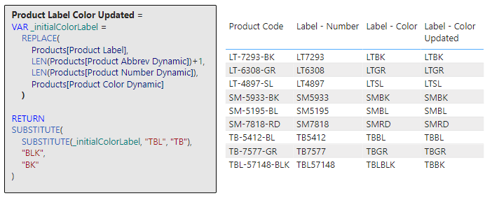
Product Label Color Updated =
VAR _initialColorLabel =
    REPLACE(
        Products[Product Label],
        LEN(Products[Product Abbrev Dynamic])+1,
        LEN(Products[Product Number Dynamic]),
        Products[Product Color Dynamic]
    )

RETURN
SUBSTITUTE(
    SUBSTITUTE(_initialColorLabel, "TBL", "TB"),
    "BLK",
    "BK"
)
Here we start by defining the variable _initialColorLabel using the same expression as the previous example. Then we refine this with a double substitution! The inner SUBSTITUTE (SUBSTITUTE(_initialColorLabel, "TBL", "TB")) takes the initial label as the main text string and searches for TBL and replaces it with TB. The result of this (i.e. TBBLK) is then used as the initial text string for the outer SUBSTITUTE, which searches this string for BLK and replaces it with BK. This produces the new label that is consistent for all products.
Now we are starting to see the true power of DAX Text Functions, this expression does so much more than just a singular adjustment: it first reshapes the product label and then it goes even further to make sure the abbreviation and color codes that make up the label are consistent and concise. It is an illustration of how DAX can incrementally build and refine results for more accurate and streamlined outputs.
Although, these examples are helpful, it may be best to perform these transformations upstream when creating the dynamic extractions. For example the Product Abbrev Dynamic column we created early:
This would ensure consistency where ever the product code is used within the report.
As we continue our journey into the realm of DAX, remember that the right tool hinges on your specific needs. While CONCATENATE and COMBINEVALUES both join text strings, their nuanced differences could significantly influence the effectiveness of your data analysis and the presentation of your data. Choose wisely!
LEN & FORMAT — The Essentials
In the realm of DAX Text Functions, while both LEN and FORMAT serve distinct purposes, they play crucial roles in refining and presenting textual data. Throughout this deep dive into DAX Text Functions, you may have noticed these functions quietly powering several of our previous examples, working diligently behind the scenes.
For instance, in our Product Color Dynamic calculated column LEN was instrumental in determining the appropriate number of characters for the RIGHT function to extract. Similarly, our Yearly Page Title measure makes use of FORMAT, to ensure an aesthetic presentation of the YTD Sales value.
These instances highlight the versatility of LEN and FORMAT, illustrating how they can be combined with other DAX functions to achieve intricate data manipulations and presentation. Let’s take a look at the details of these two essential functions.
LEN Function: provides a straightforward way to understand the length of a text string and the syntax couldn’t be more simple.
LEN(text)
The text string you wish to know the length of is represented by “, just pass this to LEN to determine how many characters make up the string. The text string of interest could also be a column reference.
Now that you are more familiar with the LEN function revisit the previous examples to see it in action.
Product Color Dynamic =
VAR _firstHyphenPosition =
    FIND (
        "-",
        Products[Product Code]
    )
VAR _lastHyphenPosition =
    SEARCH (
        "-",
        Products[Product Code],
        _firstHyphenPosition + 1
    )
RETURN
    RIGHT (
        Products[Product Code],
        LEN ( Products[Product Code] ) - _lastHyphenPosition
    )
Product Label Color =
REPLACE (
    Products[Product Label],
    LEN ( Products[Product Abbrev Dynamic] ) + 1,
    LEN ( Products[Product Number Dynamic] ),
    Products[Product Color Dynamic]
)
FORMAT Function: reshapes how data is visually represented, with this function you can transition the format of data types like dates, numbers, or durations into standardized, localized, or customized textual formats. The syntax is as follows:
FORMAT(value, format_string[, locale_name])
Here, value represents the data value or expression that evaluates to a single value you intend to format and could be a number, date, or duration. The format string, format_string, is the formatting template and determines how the value will be presented. For example a format string of 'MMMM dd, yyyy' would present a value of 2023-05-12 as May 12, 2023. The locale_name is optional and allows you to specify a locale, different regions or countries may have varying conventions for presenting numbers, dates, or durations. Examples include en-US, fi-FI, or it-IT.
Note: The result of FORMAT has a text data type, meaning that if a numeric value is formatted using FORMAT it could not then be used on visuals where the values section requires a numeric data type, or it could not be used to perform numerical calculations without converting it back to a number.
Now that you know the details of FORMAT see it put to work by revisiting the Yearly Page Title measure.
Yearly Page Title =
COMBINEVALUES (
    " ",
    YEAR (TODAY ()),
    "- Year to date sales:",
    FORMAT ([YTD Sales TOTALYTD], "Currency")
)
In this example, you see that the format_string uses a value of Currency to format the YTD sales. This is an example of a predefined numeric format. For more details on predefined numeric formats, custom numeric formats, custom numeric format characters, predefined date/time formats, and custom date/time formats visit the documentation here:
Beyond Strings: The Culmination of DAX Text Wisdom
Words share our world. And in the realm of data, they offer valuable insights. With DAX Text Functions, you have the power to manipulate, transform, and uncover these insights.
We have explored just a subset of DAX Text Functions during our journey here. There is still more to be uncovered so don’t stop learning here. Keep expanding and perfecting your DAX textual skills by exploring other text functions here:
And, remember, anyone who has never made a mistake has never tried anything new. So, don’t be afraid of making mistakes; practice makes perfect. Continuously experiment and explore new DAX functions, and challenge yourself with real-world data scenarios.
Thank you for reading! Stay curious, and until next time, happy learning.
And, remember, as Albert Einstein once said, “Anyone who has never made a mistake has never tried anything new.” So, don’t be afraid of making mistakes, practice makes perfect. Continuously experiment and explore new DAX functions, and challenge yourself with real-world data scenarios.
If this sparked your curiosity, keep that spark alive and check back frequently. Better yet, be sure not to miss a post by subscribing! With each new post comes an opportunity to learn something new.