Power BI Filter Context: Unraveling the Impact of Filters on Calculations

Series Review

One of the early stages of creating any Power BI report is the development of the data model. The data model will consist of data tables, relationships, and calculations. There are two types of calculations: calculated columns, and measures.

Check out Power BI Row Context: Understanding the Power of Context in Calculations for key differences between calculated columns and measures.

Row Context — What it is, When is it available, and its Implications

All expressions, either from a calculated column or a measure, get evaluated within the evaluation context. The evaluation context limits the values in the current scope when evaluating an expression. The filter context and/or the row context make up the evaluation context.

Power BI Row Context: Understanding the Power of Context in Calculations explores the row context in depth. While Power BI Iterators: Unleashing the Power of Iteration in Power BI Calculations explores iterator functions, which are functions that create row context.

Iterator Functions — What they are and What they do

This article is the third of a Power BI Fundamental series with a focus on the filter context. The example file used in this post is located here – GitHub.


Introduction to Filter Context

Filter context refers to the filters applied before evaluating an expression. This filter context limits the set of rows of a table available to the calculation. There are two types of filters to consider, the first is implicit filters or filters applied by the user via the report canvas. The second type is explicit filters which use functions such as CALCULATE() or CALCULATETABLE().

The applied filter context can contain one or many filters. When there are many filters the filter context will be the intersection of all the filters. When the filter context is empty all the data is used during the evaluation.

Filter context propagates through the data model relationships. When defining each model relationship the cross-filter direction is set. This setting determines the direction(s) the filters will propagate. The available cross-filter options depend on the cardinality type of the relationship. See available documentation for more information on Cross-filter Direction and Enabling Bidirectional Cross-filtering.

It is important to be familiar with certain DAX functions which can modify the filter context. Some examples used in the post include CALCULATE()ALL(), and FILTER().


The CALCULATE Function

The CALCULATE() function can add filters to a measure expression, ignore filters applied to a table, or overwrite filters applied from within the report visuals. The CALCULATE() function is a powerful and important tool when updating or modifying the filter context.

The syntax of CALCULATE() is:

CALCULATE(<expression>, <filter1>, <filter2>, ...)

Use the CALCULATE() function when modifying the filter context of an expression that returns a scalar value. Use CALCULATETABLE() when modifying the filter context of an expression that returns a table.


Exploring Filter Context

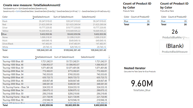
The table below is a visualization of the total sales amount for each product color.

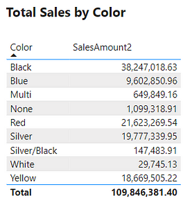
The table visual creates filter context, as seen by the total sales amount for each color or row. Evaluating SalesAmount2 occurs by first filtering the SalesOrderDetail table by the color, and then evaluating the measure with the filtered table. This is then repeated for each product color in the SalesOrderDetail table.

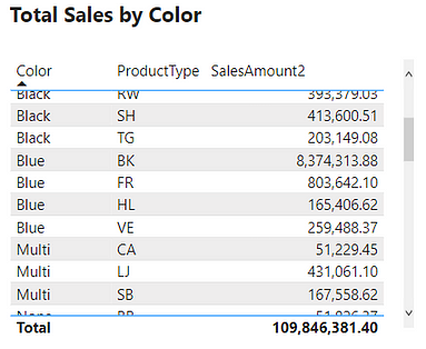
The above example only contained the single product color filter. However, as mentioned previously, the filter context can contain multiple filters. The example table below adds the ProductType to the table. The addition of this field breaks down the total sales first by color and then by product type. For each row, the underlying SalesOrderDetail table is first filtered by color and product type before evaluating the SalesAmount2 measure. In these examples, it is the table visual that is creating the filter context.


Create Filter Context with Slicers

Another way to create filter context is through the use of slicer visuals. For this example, a slicer of the ProductType is created.

When no value is selected in the slicer the filter context from the slicer visual is null. Meaning at first the card visual shows the SalesAmount2 value evaluated for all data. Additionally, when no value is selected in the slicer the only filter context is ProductColor from the table visual.

Following the selection of BK in the product type slicer, the values in both the table and the card visual are updated. The card visual now has one filter context which is the product type BK. This is evaluated by creating a filtered table and SalesAmount2 is evaluated for this filtered table.

The SalesAmount2 measure is defined by:

SalesAmount2 =
SUMX (
    SalesOrderDetail,
    SalesOrderDetail[OrderQty] * SalesOrderDetail[UnitPrice] * 
    ( 1 - SalesOrderDetail[UnitPriceDiscount] )
)

After selecting an option from the slicer the measure is re-evaluated. The re-evaluation occurs to account for the newly created filter context. The filter context creates a subset of the SalesOrderDetail table that matches the slicer selection. Then the row context evaluates the expression row-by-row for the filtered table and is summed. SUMX() is an example of an iterator function, see Power BI Iterators: Unleashing the Power of Iteration in Power BI Calculations for more details. The updated value is then displayed on the card visual.

Iterator Functions — What they are and What they do

The table visual works in a similar fashion but, there are two filters applied. The table visual has an initial filter context of the product color. After the selection of BK, the table gets updated to visualize the intersection of the product color filter and the product type filter.

Following a selection in the slicer visual, if a row in the table visual is selected this will also apply a filter. The filter context is the intersection of the table selection filters and the slicer. The updated filter context gets applied to all other visuals (e.g. the card visual).


Create Filter Context with CALCULATE

Previous examples created the filter context using implicit filters. Generally, the user creates this type of filter through the user interface. Another way to create filter context is by using explicit filters. Explicit filters get created through the use of functions such as CALCULATE(). For this example, rather than having to select BK in the slicer to view total bike sales, we will use CALCULATE(). We will create a new measure that will force the filter context. We can do this because CALCULATE() allows us to set the filter context for an expression.

We define the BikeSales measure as:

BikeSales =
CALCULATE ( 
   SalesOrderDetail[SalesAmount2], 
   Products[ProductType] = "BK" 
)
  • Expression: SalesOrderDetails[SalesAmount2]
  • Filter: Products[ProductType]="BK"

BikeSales is then added to the table visual alongside SalesAmount2. When the BK product type is the slicer selection the two table columns are equal. Both measures have the same filter context created by product color and product type. Removing the implicit product type filter by unselecting a product type updates the filter context. The SalesAmount2 expression is re-evaluated with the updated filter context. Since the filter context created by the slicer is now null the SalesAmount2 value calculates using all the data. The BikeSales values do not change. This is because of the explicit filter used by the CALCULATE() function when we defined the measure. The BikeSales measure still has the filter Products[ProductType]="BK" applied regardless of the product type slicer.

The CALCULATE() function only creates filter context and does not create row context. So an important question to ask is why or how the BikeSales measure works. The CALCULATE() function references a specific column value, Products[ProductType]="BK". Yet, the CALCULATE() function does not have row context. So how does Power BI know which row it is working with? The answer is that the CALCULATE() function applies the FILTER() function. And the FILTER function creates the row context required to evaluate the measure.

Within the CALCULATE() function the Products[ProductType]="BK filter is shorten syntax. The filter argument passed to CALCULATE() is equivalent to FILTER(ALL(Products[ProductType]), Products[ProductType]="BK")). The ALL() function removes any external filters on the ProductType column and is another example of a function that can modify the filter context.

Keep External filters with CALCULATE

The CALCULATE() function evaluates the filter context both outside of and within the function. The filter context outside of the function can come from user interaction with visuals. The filter context within the function is the filter expression(s).

To explore this we create a table with the Product Type, SalesAmount2, and SalesBike.

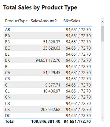
The SalesAmount2 column shows the total sales amount, if any, as expected. While the BikeSales column shows the same repeated value for all rows and is incorrect. Looking at the Product Type BK row we can see this row is correct. This table demonstrates that CALCULATE()overwrites external filters.

For example, the BB product type row filters SalesOrderDetail before evaluating SalesAmount2. This returns the correct total sales for the BB product type. When evaluating BikeSales this external product type filter gets overwritten. The measure calculates the sales amount value for the BK product type due to the explicit filter and returns this value for all rows.

Using the KEEPFILTERS() function within CALCULATE() will force CALCULATE() to keep both external and internal filters.

To do this we update BikeSales to:

BikeSales = 
CALCULATE(
   SalesOrderDetail[SalesAmount2], 
   KEEPFILTERS(Products[ProductType]="BK")
)

After updating the measure definition the resulting table is shown below.

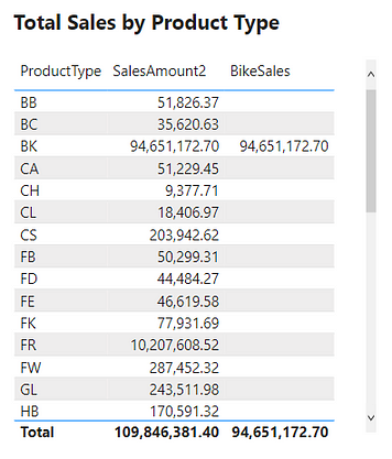
Keeping the external filters is shown by the empty values for all rows except BK. For example, we look again at the BB product type row. When evaluating BikeSales Power BI keeps the external filter Products[ProductType]="BB" and the internal filter Products[ProductType]="BK". When applying more than one filter the filter context is the intersection of the two. The intersection of the two applied filters for the BB row is empty. A product cannot be both of type BB and BK.


More CALCULATE Examples

The CALCULATE() function plays an integral part in the filter context. Below are more examples to show key concepts and show that CALCULATE() is an important part of the filter context.

Creating a measure of High Quantity Sales

For the first example, we will be creating a sales measure showing the total sales amount for high-quantity orders. Creating this measure requires first filtering the SalesOrderDetail table based on the OrderQty. Then evaluating the SalesAmount2 measure with this filtered table.

We define HighQtySales as:

HighQtySales = 
CALCULATE(
   [SalesAmount2], 
   SalesOrderDetail[OrderQty]>25
)

We then visualize this measure on a card visual and see that 96.30K of our total 109.85M sales come from a high-quantity order. This again demonstrates the filter arguments passed to CALCULATE() are shorthand syntax. The filter arguments within CALCULATE() use the FILTER() function to create the row context required. In this example SalesOrderDetail[OrderQty]>25 is equivalent to FILTER(ALL(SalesOrderDetail),SalesOrderDetail[OrderQty] > 25).

The FILTER() function is an example of an iterator function and creates the row context. The row context allows for row-by-row evaluation of the OrderQty. Meaning it evaluates SalesOrderDetail[OrderQty] > 25 for each row of the SalesOrderDetail table. FILTER() then returns a virtual tale that is a subset of the original and contains only orders with a quantity greater than 25.

Percentage of Sales by Product Color

For the second example, we will create a measure to show the percentage of total sales for each product color. To create this we will start with a new AllSales measure. AllSales uses the CALCULATE() function to remove any filters and evaluates SalesAmount2.

We define AllSales as:

AllSales = 
CALCULATE(
   [SalesAmount2], 
   ALL(Products[Color])
)

AllSales is then added to the table visual Percentage of Sales by Color. Once added the AllSales column shows 190.85M total sales value for each color. This is consistent with the SalesAmount2 card visual. Repeating this value for each color is also expected because of the filter expression ALL(Products[Color]).

ALL(Products[Color]) creates a new filter context and gets evaluated with any other filters from the visuals. In this example, CALCULATE() overwrites any external filters on Products[Color]. This is why once added to the table visual AllSales displays the total sales value repeated for each row.

The ALL() function removes any filter limiting the color column that may exist while evaluating AllSales. It is best practice to define a measure as specific as possible. Notice, in this example ALL() applies to Product[Color], rather than the entire Product table. If other filters exist on other columns from the visuals these filters will still impact the evaluation. For example, selecting a product type from the slicer will adjust all values.

Following the selection, SalesAmount2 represents the total BK sales for each color. While the AllSales measure now represents the total sales for all BK product types. This occurs because when there are multiple filters the result is the intersection of all the filters.

In this case, All(Product[Color]) removes the filter on the color column. The slicer visual creates an external filter context of only BK product types. During the evaluation, the intersection of these two creates the evaluation context.

We can also remove the external filter context created by the product type slicer. To do this, we update the AllSales measure to include Products[ProductType] as an additional filter argument.

We update the filter expression of the CALCULATE() function to:

AllSales = 
CALCULATE(
   [SalesAmount2], 
   ALL(Products[Color], 
   Products[ProductType]
)

After updating the measure the AllSales column of the table visual updates to the total sales value. The column now displays the expected 109.85M value and is no longer impacted by the filter context created by the slicer visual.

Another option to remove the filter context within CALCULATE() is to use the REMOVEFILTER() function.

AllSales = 
CALCULATE(
   SalesOrderDetail[SalesAmount2], 
   REMOVEFILTERS(
      Products[Color], 
      Products[ProductType]
   )
)

We created AllSales as an initial step of the broader goal to calculate the percentage of total sales. To calculate the percentage we will update the AllSales expression. We can do this by saving the AllSales expression as a variable within the measure. We will also create another variable to store the SalesAmount2 value, which will be the total sales for each product color. Lastly, we will update the measure name to PercentageSales which will RETURN the division of the two sales variables.

PercentageSales =
VAR Sales = SalesOrderDetail[SalesAmount2]
VAR AllSales = 
CALCULATE(
   SalesOrderDetail[SalesAmount2], 
   REMOVEFILTERS(
      Products[Color],
      Products[ProductType]
   )
)

RETURN
DIVIDE(Sales, AllSales)

Thank you for reading! Stay curious, and until next time, happy learning.

And, remember, as Albert Einstein once said, “Anyone who has never made a mistake has never tried anything new.” So, don’t be afraid of making mistakes, practice makes perfect. Continuously experiment and explore new DAX functions, and challenge yourself with real-world data scenarios.

If this sparked your curiosity, keep that spark alive and check back frequently. Better yet, be sure not to miss a post by subscribing! With each new post comes an opportunity to learn something new.

Power BI Iterators: Unleashing the Power of Iteration in Power BI Calculations

Overview

In order to facilitate analysis and visualization in Power BI a data model must first be created. The data model consists of individual data tables, relationships, and calculations. Calculations come in the form of either calculated columns or measures.

Check out this post to explore the key differences between calculated columns and measures.

Row Context — What it is, When is it available, and its Implications

The evaluation context limits the values in the current scope when Power BI evaluates a DAX expression. There are two types of evaluation context, filter and row, that can be active during the evaluation of a DAX expression.

This post is the second of a Power BI Fundamental series with a focus on iterator functions. The example file used in this post is located found on GitHub at the link below.

Power BI key fundamentals example files


Introduction

This post will build upon the Power BI file created in Part 1 of the series titled row_context_example. The example file for this post is iterator_functions, and both can be found on GitHub at the link above.

As noted at the end of Power BI Row Context: Understanding the Power of Context in Calculations, creating a measure by default was unable to reference the row values of a column. When creating a measure a column can be referenced and passed to a standard aggregation function. The standard aggregation function will return only a single aggregated value. This is not the row-by-row functionality that will be required to replace a calculated column, such as SalesAmount found in the SalesOrderDetail table.

Creating the desired measure will require an iterator function to create row context.

Understanding Iterators

An iterator moves row-by-row or iterates through an object. The object can be a data model table or a virtual/temporary table. Data model tables are tables loaded into or linked to within Power BI. A table generated from within a measure that persists only for a temporary period of time is a virtual table.

An iterator function can return a single value (e.g. number, text, date) or a virtual table. An iterator generally has two arguments:

  • The object (i.e. table) to iterate through
  • The expression evaluated for each row of the object

It can be helpful to think of the expression as a temporary column of the object. Evaluation of the expression occurs row-by-row creating a column of calculated results. The column of results only persists during the evaluation and is not loaded to the data model. The purpose of the temporary column is to calculate the final returned value of the iterator.

Examples of iterator functions include SUMXMINXMAXXAVERAGEX, and RANKX. The ending X is only a common identifier, FILTER is an example of an iterator function that does not end with a X.

Example iterator function:

SUMX(
   SalesOrderDetail, 
   SalesOrderDetail[OrderQty] * SalesOrderDetail[UnitPrice] * (1 - SalesOrderDetail[UnitPriceDiscount])
)
  • Table: SalesOrderDetail – the object iterated over
  • Expression: SalesOrderDetail[OrderQty] * SalesOrderDetail[UnitPrice] * (1 - SalesOrderDetail[UnitPriceDiscount]) – the expression evaluated for each row.

Once implementing the iterator SUMX and specifying the table as SalesOrderDetails the columns of the table will be recognized and able to be referenced like when a calculated column was created. The new measure SalesAmount2 created using an iterator will replace the calculated column SalesAmount. Comparing the default aggregation of the SalesAmount column (i.e. Sum of SalesAmount) and the new measure SalesAmount2 it can been see the values are equal.


Iterator Functions that Generate Virtual Tables

There are iterator functions such as SUMX that return a scalar value and there are ones like FILTER that return virtual tables.

To further explore, first create a new table in the data model generated by the returned table of the FILTER function.

For this example, we use the FILTER function to create a new ProductBlue table. For the first argument of the FILTER function we pass in the Product table. Then we filter that table using a filter expression defined as Products[Color] = "blue".

ProductBlue = FILTER(Products, Products[Color] = "blue")

We then can visualize this new table and compare the row count to the count of ProductID by color of the original table. Comparing these two tables we see that ProductBlue is a subset of the Product table.

The generation of this table highlights the iterating functionality and the row context when evaluating the FILTER function. To create the ProductBlue table the FILTER iterator function must create row context. During the evaluation, the function must go within the Products table and for each row (i.e. row context) evaluate what the product color is. If the color is Blue the function returns True otherwise returns False. The resulting table then consists of only rows from the original table which evaluated to a value of True.

Creating the new ProductBlue table was for demonstrative purposes. The table returned by FILTER can be a virtual table used within a measure. In this case, the ProductBlue table would only persist while the measure is being evaluated. As an example, create a new ProductBlueMeasure measure using the COUNTROWS function. COUNTROWS takes a single argument, the table to count the row of. To do this we will pass the FILTER expression used to create the ProductBlue table to the COUNTROWS function. To further demonstrate that the ProductBlue table is unnecessary, we can create a similar ProductBlackMeasure by changing =”blue" to =”black". Viewing these measures shows the result is the same counts that were produced by the other methods used to obtain this count.


Combining Iterators

More complex measures can be created by combining or nesting iterators. For example, combining the product color and the sales data, such as evaluating the total sales for only blue products. This measure will first create a virtual table of the sales data for only blue products. Then iterate row-by-row through the virtual table and evaluate the sales amount. Finally, return the total sales amount.

The DAX expression will be:

SUMX(
   FILTER(
      SalesOrderDetail, 
      RELATED(Products[Color])="Blue"
   ), 
  SalesOrderDetail[OrderQty] * SalesOrderDetail[UnitPrice] * (1 - SalesOrderDetail[UnitPriceDiscount])
)

The virtual table mentioned above is generated by FILTER(SalesOrderDetail, RELATED(Products[Color])="Blue").
This is the first iterator function that is evaluated using the SalesOrderDetail table and the expression RELATED(Products[Color])="Blue".

RELATED() is a function that returns a related value from another table. This function can be used since the Product table is related to the SalesOrderDetail table with a key value of ProductID. The FILTER function then returns a subset of the SalesOrderDetail table containing only rows where the product is blue. This virtual table is then passed to SUMX.

Then the expression evaluated row-by-row is:

SalesOrderDetail[OrderQty] * SalesOrderDetail[UnitPrice] * (1 - SalesOrderDetail[UnitPriceDiscount])

Which returns the total sales amount for each row. Then this temporary column is summed by the SUMX function.

Viewing the two tables on the left, the totals sales for the Blue products for all methods is approximately 9.60M. Selecting the blue row in the top table filters the table below, to show sales by Product for only blue products. Viewing the totals for all three methods also shows a value of approximately 9.60M. Lastly, viewing the value card under Nested Iterator shows that the above created DAX expressions results in the same value of 9.60M.

Key concepts are highlighted in the above example

  • Both SUMX and FILTER create row context
  • The FILTER function returns a virtual table which is a subset of SalesOrderDetail
  • SUMX returns the sum of the row-by-row calculation of the sale amount
  • The table passed to SUMX is the table that is returned by the FILTER function, this table only persists during the evaluation of SUMX

The concept of evaluation context has been mentioned in this post as well as in the previous post – Power BI Row Context: Understanding the Power of Context in Calculations.

Row Context — What it is, When is it available, and its Implications

Evaluation context is the context in which a DAX formula evaluates a calculation. There are two types, Power BI Row Context: Understanding the Power of Context in Calculations explored the first type, row context. This post explored iterators or specific functions which create row context to perform multi-column calculations. Check out Part Three of this series which will explore the second type of evaluation context, the filter context.

Filter Context – How to create it and its impact on measures


Thank you for reading! Stay curious, and until next time, happy learning.

And, remember, as Albert Einstein once said, “Anyone who has never made a mistake has never tried anything new.” So, don’t be afraid of making mistakes, practice makes perfect. Continuously experiment and explore new DAX functions, and challenge yourself with real-world data scenarios.

If this sparked your curiosity, keep that spark alive and check back frequently. Better yet, be sure not to miss a post by subscribing! With each new post comes an opportunity to learn something new.

Power BI Row Context: Understanding the Power of Context in Calculations


In order to facilitate analysis and visualization in Power BI a data model must first be created. The data model will consist of individual data tables, relationships between the tables, and calculations to aid in the analysis. Calculations typically come in the form of either calculated columns or measures.

A few key differences between calculated columns and measures include:

Calculated Columns:

  • Resolves as a scalar value
  • Persists in each row of a table
  • Increases the size of the data model

Measures:

  • Resolves as an aggregate value
  • Displays as a data point
  • Does not impact the size of the data model

When a DAX expression is evaluated the values the expression can access are limited by the evaluation context. When a calculated column or measure is evaluated there are two fundamental types of evaluation context: (1) Filter Context, and (2) Row Context.

This article is the first of a series focused on the key fundamentals of Power BI. This first article will focus on the concept of row context. Parts 2–4 in the series will focus on iterator functions, filter context, and context transition.


Understanding Row Context

The row context limits a DAX expression during evaluation to only the current row, the reference to each specific row is defined by the row context.

Row context exists when:

  • Creating calculated columns within a table
  • Creating iterators, see Part 2 for more details on iterator functions

Using Excel as an example, multiplying the values in two cells can be achieved with the formula =A2 * B2. The key difference is that when performing calculations in Excel the formula contains a reference to a cell defined by column A and row 2 however, in DAX there is no reference to a cell. Rather a calculation is carried out column by column [A] * [B]. DAX operates on columns and tables and it is the row context which provides the required row information for the calculation to be carried out.

The above DAX multiplication example, [A] * [B], performs the desired calculation row-by-row through the entire table. This row-by-row functionality makes the row context similar to an iterator.

See the upcoming Part 2 of the series for more details on iterator functions.

Iterator Functions — What they are and What they do


Creating a Calculated Column

As mentioned above, row context is invoked while creating a new calculated column. As an example, a new SalesAmount calculated column will be added to a SalesOrderDetail table. The example data and Power BI file can be found on GitHub.

Power BI key fundamentals example files

SalesAmount = 
SalesOrderDetail[OrderQty] * SalesOrderDetail[UnitPrice] * (1 - SalesOrderDetail[UnitPriceDiscount])

While entering the above formula, after starting to type the column names in the formula bar (e.g. OrderQtyUnitPrice, and UnitPriceDiscount) it can be seen that IntelliSense can recognize and reference the corresponding columns in the SalesOrderDetail table (e.g. SalesOrderDetail[OrderQty]).

Within the SalesAmount expression, only the column names are specified, however, since this is creating a calculated column the row context is available. This means that during the evaluation of the expression SalesOrderDetail[OrderQty] does not reference the entire column but rather the OrderQty value for the specific row within the scope of the calculation. This allows the new SalesAmount column to use the correct values when it is calculated row-by-row.

Viewing the new SalesAmount column shows that the values are calculated for each row in the table. This is because row context means to iterate over each row of the table and perform the calculation for the specific row that is in the current scope.

The new calculated column can then be utilized in creating a new measure, TotalSalesAmount

TotalSalesAmount = SUM(SalesOrderDetail[SalesAmount])

This new measure can then be included in visuals to summarize the sales data, for example, visualize the total sales by product color or by product name.

The tables above show that the new TotalSalesAmount measure for each product color/name and the sum of the SalesAmount calculated column are equal. This highlights that the new measure and the default aggregation (i.e. sum) will produce the same values.

Limitation

The method of adding a new calculated column is beneficial for aiding in understanding the impacts and use of the row context. However, a limitation to the approach of creating a column similar to SalesAmount is that each column created in a data model table increases the data model size. This is because calculated columns are created and stored as columns in the data model when the data is loaded (i.e. the .pbix file is opened or data is refreshed). Due to this, a column like SalesAmount typically would not be created in the data model, rather a measure can be used which does not increase the size of the overall data model. Measures do not increase the size of the data model because they are calculated in real-time, that is when the measure is used in a visual (table or chart).

There are certain situations where a measure cannot be used and a calculated column is required. For example, a calculated column is required when the resulting value is to be used as an axis on a visual.


Replacing a Calculated Column with a Measure

Replacing the SalesAmount calculated column with a measure may seem straightforward. Looking at the two formulas below, it is not unreasonable to think that the reference to SalesOrderDetail[SalesAmount] within the TotalSalesAmount measure could simply be replaced with the formula of the SalesAmount calculated column.

SalesAmount = SalesOrderDetail[OrderQty] * SalesOrderDetail[UnitPrice] * (1 - SalesOrderDetail[UnitPriceDiscount])
TotalSalesAmount = SUM(SalesOrderDetail[SalesAmount])

However, if you create a new measure (e.g. TotalSalesAmount2) and start typing OrderQty IntelliSense will not provide it as an option to select as it did previously when creating the calculated column.

The table columns are not available because by default a measure does not have row context. Without the row context Power BI does not know which specific OrderQty value should be referenced. For creating a measure that requires row context an iterator function will have to be used.

An iterator function can retrieve values from other columns in a table based on the row context, then perform an operation on the column values row-by-row, and finally aggregate the results.

Check out Power BI Iterators: Unleashing the Power of Iteration in Power BI Calculations for an exploration of iterators.

Iterator Functions — What they are and What they do


Thank you for reading! Stay curious, and until next time, happy learning.

And, remember, as Albert Einstein once said, “Anyone who has never made a mistake has never tried anything new.” So, don’t be afraid of making mistakes, practice makes perfect. Continuously experiment and explore new DAX functions, and challenge yourself with real-world data scenarios.

If this sparked your curiosity, keep that spark alive and check back frequently. Better yet, be sure not to miss a post by subscribing! With each new post comes an opportunity to learn something new.


From Chaos to Clarity: Revolutionize Your Inbox with Power Automate

Escape the email madness! Discover how to use Power Automate to declutter your inbox with effortless automation. Take back control of your inbox!

Power Automate offers a wide range of connectors for various services allowing for the automation of certain tasks. Managing and organizing emails is a common repetitive task that can take a fair amount of time and manual effort, and let’s face it’s not exciting work. Thankfully, Power Automate and the Outlook in Office 365 connector can provide some relief.

When searching the Power Automate connectors and actions for Outlook there is an Office 365 Outlook and an Outlook.com option. Microsoft recommends when using a work or school email account use Office 365 Outlook and when using a personal account use the Outlook.com connector

This article will provide an overview of the Outlook in Office 365 connector and some examples of how it can be used to conduct an Inbox Cleanup task.

Office 365 Outlook Actions

The Office 365 Outlook connector offers several actions or events that the Power Automate workflow could do — List of Office 365 Outlook Actions — below shows just a partial list.

Automating an Outlook inbox cleanup task will focus on the following actions.

Get emails (V3)

This action will retrieve emails from a folder (e.g. Inbox). This action can be configured to fetch both read and unread emails.

Move email (V2)

This action will move an email to the specified folder, within the same mailbox.

Using the low-code interface the specified folder must be selected, to dynamically set the destination folder based on the characteristics of the email the folder ID must be specified, see below for details.

The Basics

To get started the workflow will fetch up to 10 emails, and process them based on the Read status. Unread emails will be moved to the Unread folder and Read emails will be moved to the Read folder.

Flow Diagram

Power Automate Flow

To start the Power Automate flow the trigger is defined, here it is a manual trigger, but could be scheduled. Following this, a noEmails variable is defined to be used to exit the Do until loop which will continue to fetch 10 email batches from the inbox until there are no more emails ( noEmails = True). After initializing the variable the Do until flow control is added.

Within the Do until loop, there are 3 main events:

  1. The Get emails action retrieves the top 10 emails from the Inbox. To configure this action, select the folder to retrieve the emails from, and then for this flow the Fetch Only Unread Messages was set to No and the Top option was set to 10 (pictured above in the Get emails (V3) section).
  2. Determine if there are emails to process and set the noEmails variable to the appropriate True or False value. The set variable value is determined by the expression: if(equals(length(outputs('Get_emails_(V3)_from_Inbox')?['body/value']),0), true, false)
  3. The For Each Email loop iterates over each of the retrieved emails and moves the emails to the appropriate folder based on the email’s read status.

The For Each Email control structure applies the actions contained within it to each of the emails retrieved by the Get emails action.

Limitations

A limitation of the above flow is that the destination folder for the Move email actions had to be explicitly selected. This will likely be fine if there are only a few potential mailbox folders, however, can easily become unmanageable when the number of potential Inbox folders grows.

This limitation can be addressed by using Id:: <folder_id> for the Folder option within the Move email action. This solution comes with two main points to address:

  1. Where to find the Outlook folder IDs
  2. How to store/search for the folder IDs based on specific email characteristics (e.g. from specific people or domains).

Outlook Inbox Cleanup Workflow

The first example shown in this article explicitly selected the destination folder, in this example, the folder display names and IDs will be stored in an object variable. The workflow will then process the email, identifying which property from the object variable should be retrieved. Then the returned value (the folder ID) will be used in the Move email action. In this example, an object variable was used to store the display name and folder IDs, a Microsoft List could also be used. Retrieving the folder ID using this option would require a Get items action with the appropriate filter query.

Workflow Diagram

Outlook Folder Setup

The outlook mailbox used by this flow has the following folders to which the emails will be moved from the inbox. Internal emails will be moved into the Departments subfolder based on the sender’s department. External emails will be moved into the External subfolder based on the sender’s domain.

Get Folder IDs

Getting the folder IDs of an Outlook mailbox folder can involve using the Microsoft Graph API or using the peak code setting within Power Automate. Using Microsoft Graph can be a bit more advanced but still approachable when manually retrieving the folder IDs using peak code is unmanageable.

Peak Code

This method requires manually identifying each destination folder’s ID and adding it to the object variable. This can be an appropriate method when the number of destination folders is low and does not change frequently. The organizing of emails in this example primarily focuses on sorting into department folders which can be a good use case for this method because the number of departments in an organization is likely to be relatively stable.

The Move email action, shown below, shows that the folder is selected (HR).

After selecting the destination folder, in the upper right of the action select the ellipses and then Peak code.

This will reveal the inputs to this action. Under the parameters property, the folderPath can be seen. What is required to be stored for this flow is the entire folder path following Id::, this ID and the folders display name are what is stored and accessed by the workflow. See the Power Automate Flow – Variable section for an example.

Microsoft Graph

When using the Microsoft Graph approach Graph Explorer is a helpful tool. This method can also be used to get the display names and IDs of child folders. See the Power Automate Flow — Microsoft Graph section for an example.

Power Automate Flow — Variable

Again the workflow is started with a manual trigger but could be set to a scheduled trigger. The first few actions of the flow initialize four variables utilized by the flow: noEmailsfolderIDspropertyName, and sorted.

  • noEmails: boolean variable used to exit the Do until loop which continues to retrieve emails from the Inbox until noEmails=True
  • folderIDs: an object variable that stores a folder’s display name (key) and folder id (value)
  • propertyName: string variable used to get the corresponding folderIDs from the folderIDs object
  • sorted: boolean variable used to determine if the current email has been sorted by a prior step

The Do until noEmail=True is a Do until flow control action which will continue to process and sort emails in the Inbox until there are no more emails to be processed. This contains the same three actions that were described above Get emails, determine if there are emails to process, then process each email. The For Each Email loop is where a majority of the Inbox management actions occur.

The For each loop contains 4 main steps:

  1. Get the current email object, this will make attributes of the email accessible through dynamic content
  2. Set the sorted variable to False and split the From email address into the domain and the user id (everything after @ and everything before @)
  3. Move Unread emails into an Unread folder. These will be moved back to the Inbox after all emails have been processed
  4. Check if the email was sorted into the Unread folder and if not evaluate email characteristics and move the email to the appropriate folder

Action Step #1

The first step gets the current email and makes the properties of the email accessible through dynamic content.

Action Step #2

This step consists of setting the sorted value and two Compose data operations which splits the From email address into two parts, before the and after. The output of these two actions will be used to determine if the email came from an internal source which will be sorted by the sender’s department or an external source which will be sorted by domain.

The inputs expressions used are:

  • Compose — Domain: last(split(outputs('Get_email_(V2)_-_Current_Email_Object')?['body/from'], '@'))
  • Compose — User Id: first(split(outputs('Get_email_(V2)_-_Current_Email_Object')?['body/from'], '@'))

Action Step #3

This set of actions uses a Condition flow control to check the Is Read status of the current email. If False the email is moved to an Unread folder to be moved back to the Inbox folder later in the flow and sorted is set to True. If True no action is taken and the flow moves to the next set of actions.

Action Step #4

This step carries out the processing and sorting of each of the read emails. First, the flow checks the value of sorted, if sorted equals True no additional actions are taken, if False the email is sorted based on the attributes of the email.

When sorting actions are needed (sorted = False) the first action is another Condition flow control which checks if the Domain is equal to an internal domain.

If the above condition is met the email is sorted into a department folder by searching for the user profile of who sent the email using the Office 365 connector and setting the propertyName variable equal to the department attribute. Then the folder argument of the Move email action is set to:

variables('folderIds')?['departments'][variables('propertyName')].

It is important to note that the folder ID in the Move email actions is preceded by Id::

If the above condition is not met, the email is sorted by domain. This sorting involves three steps. First, a compose action is used to get the folderID of the corresponding domain folder with the inputs argument set to:

variables('folderIds')?['domain'][variables('propertyName')]

This is then followed by two Move email actions that have different configure after run settings. The Sorting Needed action is configured to run only when the compose Get propertName action fails (i.e. a property matching the domain does not exist in the folderIDs variable) and the email is moved into a Sorting Needed folder to be manually sorted.

The following External Sorting action is configured to run only when the Sorting Needed action is skipped (i.e. the Get propertName action was successful). The folder argument of the Move email action is set to the same expression as the above Get propertyName action.

After all emails in the Inbox have been processed the flow retrieves all emails that were moved to the Unread folder and moves them back to the Inbox.

Limitations

A main advantage of the approach is that the destination folder can be dynamically set without nesting Condition flow controls. However, this approach may become unmanageable if the destination folders change or if new folders are frequently added. To continue sorting into new folders would require a manual update of the folder name and ID storage source (variable or Microsoft List).

Power Automate Flow — Microsoft Graph

This approach has the same general layout as the previous flow, the only difference occurs within the Check if Internal Email flow control.

Here there are additional actions: Send an HTTP requestParse JSON, and For Each Child Folder.

The Send an HTTP request Outlook action requires a URI this can be explored and created using the Graph Explorer tool. The generalized query used here is:

https://graph.microsoft.com/v1.0/me/mailFolders/childFolders

The returned body of this action is then parsed with the Parse JSON action which allows properties of child folders (folders within Department and External) to be utilized as dynamic content.

The Schema of the Parse JSON action can be generated from a sample by testing the workflow before adding this action. Following the test, the output of the Send an HTTP request can be copied, then add the Parse JSON action and paste the output into the Insert a sample JSON Payload dialog box

After these actions, there is a For Each flow control that iterates through each child folder and compares the display name of the folder with the department of the sender. If the two are equal the folderID variable is set to the id of the corresponding folder.

The folderID variable is then used in the following Move email action in the same way as the prior flow example.

The False branch of the Check if Internal Email operates in the same way, with the only changes being there is no need to search for users (external email) and the <ParentFolderID> in the Microsoft Graph query is the folder ID corresponding to the External folder, rather than Department.

Summary

This article covered various approaches using Power Automate to automate Outlook inbox cleanup and management. The three approaches shown in the article covered a basic application of sorting emails into a Read and Unread folder. The main limitation of this flow is that the destination folder was explicitly selected and set. The following two approaches in the article covered two methods of addressing this limitation by using a variable object and querying the folders present using Microsoft Graph.


Thank you for reading! Stay curious, and until next time, happy learning.

If this sparked your curiosity, keep that spark alive and check back frequently. Better yet, be sure not to miss a post by subscribing! With each new post comes an opportunity to learn something new.